Introduction

Vision is a fundamental interface to the world, and it has become a crucial component in the development of intelligent systems. The field has deep and attractive scientific problems, which have been advancing at a rapid pace in the past few years.
In the early days of research, the focus in vision was on engineering “good” features coupled with a optimisation algorithm or a shallow neural network. As the processors became more powerful, the emphasis shifted to end-to-end approaches with inclusion of self-supervision and multi-modal learning paradigms.

It is often helpful to breakdown the perception tasks into known-algorithms. For example, in autonomous driving, the tasks include SLAM (visual, Structure from Motion), path planning (lane detection, obstacle detection, 3D localization), Semantic segmentation etc. Similarly, the tasks in augmented reality devices are gaze tracking, material and lighting estimation, head pose estimation, depth estimation, etc.

Deep learning has opened new areas of research in vision. Features such as generation of high-quality content, end-to-end training, data-driven priors and highly parallelizable architectures have proven advantageous for many problems in computer vision. However, it is also important to note the limitations of these techniques -

• Large scale labeled data is not always available
• Lack of generalization to unseen domains
• Good at narrow “classification”, not at broad “reasoning”
• Lack of interpretability
• Lack of reliability, security or privacy guarantee

To counter these problems, we typically couple our algorithms with self-supervision, physical modelling, multi-modal learning and foundation models. In the recent years, these techniques have been applied to various problems, and the following are arguably the biggest advances in Computer Vision -

• Vision Transformers
• Vision-Language Models
• Diffusion Models
• Neural Rendering

These techniques show promise to solve keystone problems in augmented reality, interactive robotics, and autonomous driving. The course will cover the following these topics, along with other fundamentals required.

• Neural Architectures

• Generative Models

• Structure from Motion

• Object Detection

• image Segmentation

• Prediction and Planning

• Inverse Rendering

• 3D GANs

• Vision-Language

Neural Architectures

The motivation for an artificial neuron (perceptron), comes from a biological neuron where the output is linear combination of the inputs combined with a non-linear activation function. From here, we develop multi-layer networks which are again motivated from the Hubel and Weisel’s architecture in biological cells.

Neural Networks

The simplest neural network is a perceptron represented by \(\sigma (x) = \text{sign}(\sum_i w_i x_i + b)\) where the optimal weight values are obtained using an unconstrained optimization problem. These concepts can be extended for “Linear Regression” and “Logistic Regression” tasks.

Non-linearity in neural networks is introduced through Activation functions such as

• Sigmoid - Have vanishing gradient issues
• tanh - Centered version of sigmoid
• ReLU - Simplest non-linear activation, with easy gradient calculation.
• ELU - Added to prevent passive neurons.

At the output layer, we apply a final non-linear function is applied to calculate the loss in the predicted output. Typically for classification problems, Softmax function is used to map the network outputs to probabilities. One-hot representations are not differentiable, and are hence not used for this task. In image synthesis problems, the output layer usually has \(255*sigmoid(z)\).

Theorem (Universal function approximators): A two-layer network with a sufficient number of neurons can approximate any continous function to any desired accuracy.

Width or Depth? A wider network needs more and more neurons to represent arbitrary function with high enough precision. A deeper network on the contrary, require few parameters needed to achieve a similar approximation power. However, “overly deep” plain nets do not perform well. This is due to the vanishing gradient problem, wherein we are not able to train deep networks with the typical optimization algorithms.

Convolution Networks

The neural network architecture is modified for images using “learnable kernels” in convolutional neural networks. Each convolution layer consists of a set of kernels that produce feature maps from the input. These feature maps capture the spatial and local relationships in the input which is crucial for images.

The induction bias in images is that neighbouring variables are locally correlated. An image need not be 2D, it can consist of multiple channels (RGB, hyperspectral, etc.), and convolutional layers work across all these channels to produce feature maps.

In a classical neural network, each pixel in the input image would be connected to every neuron in the network layer leading to many parameters for a single image. Using kernels, we use shared weights across all pixel locations, and this greatly reduces the number of learnable parameters without losing much information.

Convolution layers are generally accompanies with Pooling layers which do not have any learnable parameters, and are used to reduce the size of the output. These layers are invariant to small (spatial)transformations in the input and help observe a larger receptive field in the next layer. The latter property is important to observe hidden layers in the feature maps.

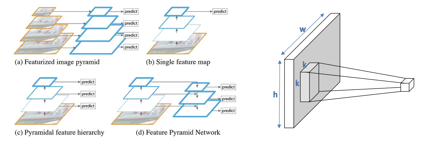
Receptive Field - It is the area in the input iamge “seen” by a unit in a CNN. Inits with deeper layers will have wider receptive fields whereas wider receptive fields allow more global reasoning across entire image. This way, the pooling leads to more rapid widening of receptive fields. We need \(\mathcal O(n/k)\) layers with \((k \times k)\) convolutional filters to have a receptive field of \(n\) in the input. Dilation layers are used to achieve the same receptive field with \(\mathcal O(\log n)\) layers.

However, in practice, the empirical receptive fields in the deeper networks is lower than the theoretical value due to sparse weights.

Convolution networks are augmented with dense layers to get the output, to learn from the feature maps.

The vanishing gradient problem in deeper networks has been solved using skip connections wherein the features from the earlier layers are concatenated with the deeper ones to allow passage of information. This way, we provide the network with the original input allowing it to learn the smaller fluctuations in the input (rather than focusing on learning the input itself).

In summary, the key operations in convolutional layers are

Input image -> Convlution -> Non-linearity -> Spatial Pooling -> Feature Maps

CNNs have the above set of operations repeated many times. CNNs have been successful due to the following reasons

• Good Abstractions - Hierarchical and expressive feature representations. Conventional image processing algorithms relied on a pyramidal representation of features, and this methodology has also paved its way in CNNs.
• Good inductive biases - Remarkable in transferring knowledge across tasks. That is, pretrained networks can be easily augmented with other general tasks.
• Ease of implementation - Can be trained end-to-end, rather than hand-crafted for each task, and they can easily be implemented on parallel architectures.

The key ideas -

• Convolutional layers leverage the local connectivity and weight sharing to reduce the number of learnable parameters.
• Pooling layers allow larger receptive fields letting us capture global features.
• Smaller kernels limit the number of parameters without compromising the performance much. This design decision comes from preferring deeper networks over wider networks. For example, \((1 \times 1)\) kernels are reduce the dimension in the channels dimension.
• Skip connections allow easier optimization with greater depth.

Why are (1, 1) kernels useful? Use fewer channels instead?

Transformers

Transformers have shown better results in almost every task that CNNs have shone previously in. CNNs require significant depth or larger kernels to share information between non-local spatial locations (recall receptive fields).

Many tasks, such as question-answering, require long-range reasoning and transformers are very good at this. For example, placing objects in augmented reality requires reasoning about light-sources, surface estimation, occlusion/shadow detection, etc. This is the primary intuition behind attention mechanism which is representative of foveated vision in humans.

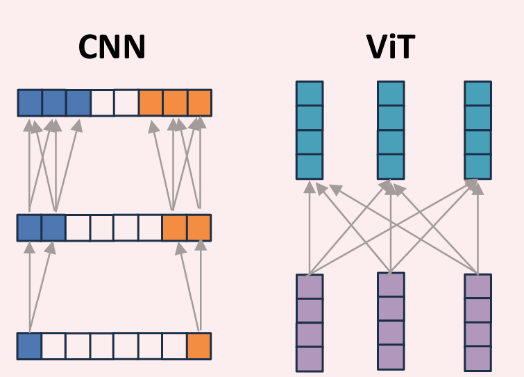
Tokens - A data type than can be understood as a set of neurons obtained from vectorizing patches of an image. Typically need not be vectors, but they can be any structured froup that alows a set of differentiable operations. Note that these tokens in hidden layers might not correspond to pixels or interpretable attributes.

The following captures a very good intuition for transformers.

A transformers acts on tokens similarly as neural network acts on neurons. That is, combining tokens is same as for neurons, except tokens are vectors \(t_{out }= \sum_i w_i t_i\). In neural networks, linear layers are represented by \(x_{out} = W x_{in}\) and \(W\) is data-free, whereas in transformers, \(T_{out} = AT_{in}\), \(A\) depends on the data (attention). Again, non-linearity in neural networks is implemented via functions like ReLU whereas transformers use dense layers for non-linearity (applied token wise).

The attention layer is a spsecial kind of linear transformation of tokens, wherein the attention function \(A = f(.)\) tells how much importance to pay to each token depending on the input query and other signals. Attention-maps help us visualize the global dependencies in the information. The required information is embedded in some dimension of the token representation. For example, the first dimension can count the number of horses in an iamge, and the bottom 3 dimensions can encode the color of the horse on the right. Attention has this flexibility to different allocations address different parts of a query. They can “attend” to only certain patches which are important to the query. This kind of functionality is difficult with CNNs.

Apply embedding and neural network (before CNNs and Transofrmers)? Same number of parameters? Essentially similar thing? Associated higher weight to more related embedding.

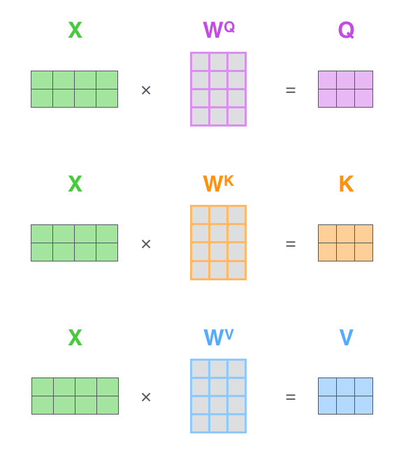
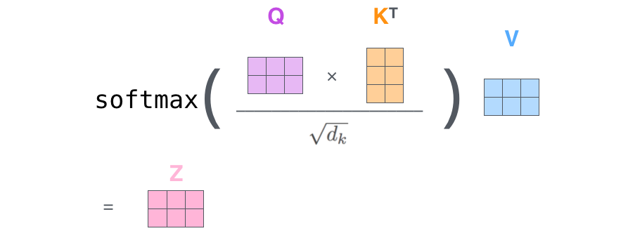
Query-Key-Value Attention

The mechanisms described previously are implemented by projecting tokens into queries, keys and values. Each of these are a vector of dimensions $p$, where $p < d$. The query vector for the question is used to weigh the key vector for each token to obtain the values. This is done via computing the similarity between query and each key, and then the attention is given by the extent of similarities, normalized with softmax. The output token is obtained by summing all value vectors with weights assigned from the previous calculations. Roughly, the process looks like -

\[\begin{align*} \left. \begin{align*} q = W_q t \\ K_i = W_k t_i \end{align*} \right\} \implies s_i = q^T k_i \\ a_i = softmax(s_i) \\ t_{out} = \sum a_i v_i \end{align*}\]

The purpose of “values” is to ‘project’ back the similarities between queries and keys to the ‘token space’.

Also note that, if the patch-size is too large, then we might lose the information within the patches. This is a tradeoff, and the decision is made based on the task at hand. For example, classification may work with large patches but tasks such as segmentation may not.

Self-Attention

How do we learn implicit representations that can work with general queries? We compute self-attention using the image tokens as the queries - information derived from the image itself. How does this process help us? For example, if we are performing instance segmentation of an image with horses. Then, the concept of ‘horse’ is learned by attending more to tother horse tokens and less to background. Similarly, ‘a particular instance’ is learned by attending less to the tokens from other horses. When we do this for all pairs across \(N\) tokens gives us an \(N \times N\) attention matrix.

Typically, this matrix is computed in the encoder part of a transformer. This matrix is then used in the decoder with an input query to obtain the required results.

Encoders

An encoder of a transformer typically consists of many identical blocks connected serially with one another. Each such encoder block, computes a self-attention matrix and passes it through a feed-forward neural network, and they need to be applied across all the tokens in the input. Since the embeddings of tokens are independent of one another, each level of encoder blocks can be applied in parallel to all the tokens (patches in vision transformers) to obtain the embeddings. Such parallel computations were not possible in previous models like RNNs, which heavily relied on sequential dependencies.

The original transformers paper normalizes the similarities with \(\sqrt{N}\) where \(N\) is the embedding dimension. This allows the gradients to stabilise and gives much better performance. This a simplified view of the mechanisms used in transformers.

In addition to these, transformers also use positional encoding to encode the position of the tokens in the input sequence. In the context of images, is encodes where each patch occurs in the image.

Positional encoding is usually done via sinusoidal functions. Other “learning-based” representations have been explored but they don’t have much different effect. This encoding structure allows extrapolation to sequnce lengths not seen in training.

They also have multi-head attention which is equivalent to multiple channels in CNNs. That is, it allows patches to output more than one type of information.

This blog explains these mechanisms in-depth for interested readers. In summary, the functions of the encoder is visualized as

Decoders

A decoder block is similar to an encoder block, with auto-regressive . The attention values learned in Encoders are used as ‘keys’ in the decoder attention block. This is called as cross attention.

Vision-Transformers

Vision transformers build on the same ideas used in a transformer. Typically, they use only the encoder part of the architecture where patches are extracted from images and are flattened to form the tokens for the attention mechanism. They are usually projected using a linear layer or a CNN before performing the calculations. Apart from this, vision transformers also include an additional class token in the embeddings to help learn the global information across the image.

CNNs typically have better inductive bias whereas transformers excel in shorter learning paths for long-range reasoning. However, the cost of self-attention is quadratic in the image size. Also note that, if the patch-size is too large, then we might lose the information within the patches. This is a tradeoff, and the decision is made based on the task at hand. For example, classification may work with large patches but tasks such as segmentation may not.

Swin Transformers and Dense Prediction Transformers

The vanilla vision transformer is restricted to classification tasks and is not optimal for other tasks like detection and segmentation. Also, as we have noted before, the quadratic complexity limit the number of patches in the image. Some image processing pipelines extract features across different scales of an image whereas the vanilla transformer is restricted to the uniform (coarse) scale.

To address these limitations, swin transformers bring two key ideas from CNNs

• Multi-scale feature maps - Feature maps from one resolution are down sampled to match the size in the next block.

  

• Local connectivity -

  • Windowed self-attention - Limit the computations by considering a local window (this was actually left as future work in the original attention paper).

  • Shifted window self-attention - Allows windowed self-attention to learn long-range features using “shifts”. Essentially, we move the patches around to bring farther patches close together.

However, these modifications are not enough for tasks like segmentation, which require reasoning at a pixel-level. Instead, we use something called as a dense prediction transformer (DPTs) where we couple the transformer encoder with a convolutional decoder to upsample and predict the required output.

CNNs are shift-invariant whereas ViTs are permutation invariant. Why?

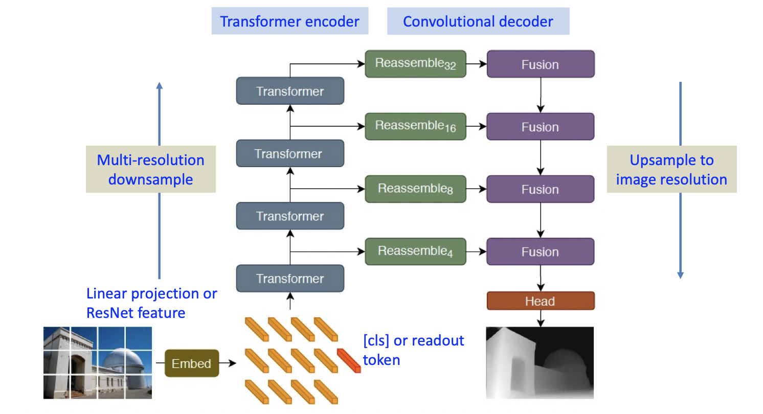
At each scale level in the above picture, we reassemble the tokens by concatenating and convolving with appropriate kernels to recover image-like representations in the decoder layers.

Multimodality

Transformers allowed for easy multi-modal representations by tokenizing data from each modality with its own variant of patches. Works such as VATT have explored merging audio waveforms, text and images.

Generative Models

Discriminative and Generative Models

Discriminative models (classifiers) learn a many-to-one function \(f\) to learn labels for a given input. A generative model \(g\) maps these labels to the input space, and this function is one-to-many since one label can map to multiple inputs. It is difficult to model a stochastic function. Therefore, a generator model is coupled with a noise vector to construct a deterministic \(g\) with stochastic input \(z\). This variable \(z\) is called a latent variable since it is not observed in training data composed of \(\{x, y\}\) pairs.

\[\begin{align*} \text{Discriminative Models learn } P(Y \vert X) \\ \text{Generative Models learn } P(X, Y) \\ \text{Conditional Generators learn } P(X \vert Y) \\ \end{align*}\]

Let us focus on image generative models. Then, each dimension of the latent variable can encode the various characteristics of the image essentially allowing us to generate a wide variety of images. The labels \(y\) for images need not be classification labels, but textual descriptions can also be used for supervision.

To understand how these models work, consider the case of unconditional generative models. The goal is, given the real data \(x\), to generate synthetic data \(\hat x\) that looks like the real data. How do we quantify ‘looks like’?

• We can try and match some marginal statistics - mean, variance, edge statistics, etc of the real data. Such measures are very useful in techniques for texture synthesis. For example, Heeger-Bergen texture synthesis [1995] uses an iterative process starting from the Gaussian noise and matches intensity histograms across different scales. Such design choices are used in modern techniques like StyleGANs and Diffusion models.

• Have a high probability of success under a model fit to real-data (A discriminator).

The key-challenge in these models is novelity in the generation to ensure generalization.

Generative models are classified into the following approaches -

• Energy-based models - Learn a scoring function \(s:X \to R\) that scores real-samples with a high score which represents energy/probability. During generation, return samples which have a high score. This paradigm is particularly useful for applications like anomaly detection.

• Sampling from Noise - Learn a generative function \(g: Z \to X\) without needing to learn a probability density function. These methods explicitly model the data distribution, and techniques like GANs and Diffusion Models come under this regime.

Density/Energy based models

Learn a scoring function \(s:X \to R\) that scores real-samples with a high score which represents energy/probability. During generation, return samples which have a high score. This paradigm is particularly useful for applications like anomaly detection.

In these methods, we produce \(p_\theta\) fit to the training data by optimizing \(\arg\min_{p_\theta} D(p_{\theta}, p_{data})\). Since we don’t know \(p_{data}\) explicitly (we only have access to samples \(x \sim p_{data}\)), we minimize the KL-divergence to reduce the distance between the distributions using the samples.

\[\begin{align*} p_\theta^* &= \arg\min_{p_\theta} KL(p_{data} \vert\vert p_\theta)\\ &= \arg\max_{p_\theta} \mathbb E_{x\sim p_{data}}[\log p_\theta] - \mathbb E_{x\sim p_{data}}[\log p_{data}] \\ &= \arg\max_{p_\theta} \mathbb E_{x\sim p_{data}}[\log p_\theta] \end{align*}\]

Intuitively, this way of optimization increases the density where the models are observed.

The energy-based models have a slight modification wherein the energy function \(E_\theta\) is unnormalized unlike the probability density function \(p_\theta\). Indeed, \(p_\theta\) can be determined as

\[\begin{align*} p_\theta &= \frac{e^{-E_\theta}}{Z(\theta)}, \\ &\text{ where } Z_\theta = \int_x e^{-E_{\theta}(x)} dx \end{align*}\]

This formulation is called as Boltzmann or Gibbs distribution. Learning energy function is convenient since normalization is intractable since we cannot see all the samples in the distribution. What is the motivation to use exponential functions?

1. It arises naturally in physical statistics

2. Many common distributions (Normal, Poisson, …) are modeled using exponential functions.

3. Want to handle large variations in probability

Although we don’t have the probabilities, we can still compare different samples using ratios of their energies.

After obtaining the energy distribution, how do we use it to sample in these approaches? Sampling approaches Markov Chain Monte Carlo (MCMC) only require relative probabilities for generating data. We can also find data points that maximize the probability.

\[\nabla_x \log p_\theta(x) = -\nabla_x E_\theta(x)\]

On the other hand, where would be prefer probability formulation over energy? Certain systems like safety in autonomous driving require absolute quantifiable probabilities rather than relative scores.

In probability modeling, the probability of space where no samples are observed is automatically pushed down due to normalization. However, in energy based models, we need an explicit negative term to push energy up where no data points are observed. To do so, we set up an iterative optimization where the gradient of the log-likelihood function naturally decomposes into contrastive terms

\[\begin{align*} \nabla_\theta \mathbb E_{x \sim p_{data}} [\log p_\theta(x)] &= \frac{1}{N}\nabla_\theta\sum_{i = 1}^N (\underbrace{-E_\theta(x^{(i)})}_{\text{ data samples}} + \underbrace{E_\theta(\hat x^{(i)})}_{\text{model samples}}) \\ &= - \mathbb E_{x \sim p_{data}} [\nabla_\theta \mathbb E_\theta (x)] + \mathbb E_{x \sim p_\theta} [\nabla_\theta \mathbb E_\theta(x)] \end{align*}\]

Sampling

We randomly initialize \(\hat x_0\) at \(t = 0\). Then, we repeat the following

1. Let \(\hat x' = \hat x_t + \eta\)$ where \(\eta\) is some noise

2. If \(\mathbb E_\theta(\hat x') < \mathbb E_\theta(\hat x_t)\), then choose \(\hat x_{t + 1} = \hat x'\).

3. Else choose \(\hat x_{t + 1} = \hat x'\) with probability \(e^{(\mathbb E_\theta(\hat x_t) - \mathbb E_\theta(\hat x'))}\)

In practice, this algorithm takes a long time to converge. A variant of this called Langevin MCMC uses the gradient of the distribution to accelerate the sampling procedure

1. Choose \(q(x)\) an easy to sample prior distribution.

2. Repeat for a fixed number of iterations \(t\)

   \[\hat x_{t + 1} \sim \hat x_t + \epsilon \nabla_x \log p_\theta(\hat x_t) - \sqrt{2\epsilon} z_t\]

   where \(z_t \sim \mathcal N(0, I)\). When \(\epsilon \to 0\), and \(t \to \infty\), we have \(\hat x_t \sim p_\theta\)

Sampling from Noise

Diffusion Models

The intuition for these models builds from our previous approach. It is hard to map pure noise to \(x \sim N(0, I)\) to structured data, but it is very easy to do the opposite. To readers familiar with autoregressive models, where we remove one pixel of information at a time, diffusion models generalise this notion further. Diffusion models have two steps in training -

The forward process in these models involves adding noise to the image \(x_0\) over many time steps. At time \(t\), we add noise \(\epsilon_t\) to obtain \(x_{t + 1}\) from \(x_{t}\). The noise addition is modeled with respect to the following equation

\[x_t = \sqrt{(1 - \beta_t) x_{t - 1}} + \sqrt{\beta_t}\epsilon_t, \quad \epsilon_t \sim N(0, I)\]

If this process is repeated for a large number of times, it can be shown that the final output simulates white noise. Now, in the learning part, we train a predictor to learn denoising from \(x_t\) to \(x_{t - 1}\). That is, given our model \(f_\theta\)

\[\hat x_{t - 1} = f_\theta(x_t , t)\]

Forward Noising

Given an image \(x_0 \sim q(x)\), we essentially add the following Gaussian noise in \(T\) time steps

\[q(x_t \vert x_{t - 1}) = \mathcal N(x_t ; \sqrt{1 - \beta} x_{t - 1}, \beta_t I)\]

The term \(\beta_t\) is referred to as the schedule and \(0 < \beta_t < 1\). Typically, we set it to a small value in the beginning and do linear increments with time. The above process is a Markov’s process, resulting in the following property

\[q(x_{1:T} \vert x_0) = \prod_{t = 1}^T q(x_t \vert x_{t - 1})\]

Instead of a slow step-by-step process, training uses samples from arbitrary time step. To decrease the computations, we use the following properties of Gaussian distributions

• Reparameterization trick: \(\mathcal N(\mu, \sigma^2)= \mu + \sigma \epsilon\) where \(\epsilon \sim \mathcal N(0, I)\)

• Merging Gaussians \(\mathcal N(0, \sigma_1^2 I)\) and \(\mathcal N(0, \sigma_2^2 I)\) is a Gaussian of the form\(\mathcal N(0, (\sigma_1^2 + \sigma_2^2) I)\)

Define \(\alpha_t = 1 - \beta_t\), and \(\bar \alpha_t = \prod_{i = 1}^t \alpha_i\), we can now sample \(x_t\) at an arbitrary time step

\[\begin{align*} x_t &= \sqrt{\alpha_t} x_{t - 1} + \sqrt{1 - \alpha_t}\epsilon_{t - 1} \\ &= \sqrt{\alpha_t\alpha_{t - 1}} x_{t - 1} + \sqrt{1 - \alpha_t\alpha_{t - 1}}\epsilon_{t - 1} \\ &\dots \\ &= \sqrt{\bar \alpha_t}x_0 + \sqrt{1 - \bar \alpha_t}\epsilon \end{align*}\]

When we schedule \(\beta_t\) such that \(\beta_1 < \beta_2 < \dots, \beta_T\) so that \(\bar \alpha_1 > \dots, > \bar \alpha_T\), such that \(\bar \alpha_T \to 0\), then

\[q(x_T \vert x_0) \approx \mathcal N(x_T; 0, I)\]

The intuition is that the diffusion kernel is a Gaussian

\[q(x_t) = \int q(x_0, x_t) dx_0 = \int q(x_0) q(x_t \vert x_0) dx_0\]

There are theoretical bounds showing a relation between the number of steps and overfitting of the model to the distribution. There are no such guarantees for VAEs.

The increasing \(\beta_t\) schedule sort of accelerates the diffusion process wherein we simulate white noise with few iterations. However, the stable diffusion paper to generate images chose the cosine learning schedule which gave better results.

Reverse Denoising

The goal is to start with noise and gradually denoise to generate images. We start with \(x_T \sim \mathcal N(0, I)\) and sample form \(q(x_{t - 1} \vert x_t)\) to denoise. When \(\beta_t\) is small enough, we can show that this quantity is a Gaussian. However, estimating the quantity is difficult since it requires optimization over the whole dataset.

Therefore, we learn a model \(p_\theta\) to reverse the process

\[P_\theta(x_{t - 1} \vert x_t) = \mathcal N(x_{t - 1}; \mu_\theta(x_t, t), \Sigma)\]

#

Essentially, the training objective is to maximise log-likelihood over the data distribution. A variational lower bound can be derived and is used in practice

\[\mathbb E_{q(x_0)}[-\log p_\theta(X_0)] \leq \mathbb E_{q(x_0) q(x_{1:T}\vert x_0)} \left[-\log \frac{p_\theta (x_{0:T})}{q(x_{1:T} \vert x_0)}\right]\]

Then, this decomposes into

\[\sum_{t > 1} D_{KL} (q(x_{t - 1} \vert x_t, x_0) \vert\vert p_\theta(x_{t - 1} \vert x_t)) + \text{other terms}\]

The idea is that $q(x_{t - 1} \vert x_t, x_0)$ is tractable even though $q(x_{t - 1} \vert x_t)$ is not. That is because

\[\begin{align*} q(x_{t - 1} \vert x_t, x_0) &= \mathcal N(x_{t - 1}; \tilde \mu_t(x_t, x_0), \tilde \beta_t I) \\ \text{where } \tilde \mu_t(x_t, x_0) &= \frac{\sqrt{\bar \alpha_{t - 1}}}{1 - \bar \alpha_t}x_0 + \frac{\sqrt{1 - \beta_t} ( 1- \bar\alpha_{t - 1})}{1- \bar\alpha_{t - 1}}x_t \\ &=\tilde \beta_t = \frac{1 - \bar \alpha_{t - 1}}{1 - \bar \alpha_t} \beta_t \end{align*}\]

Generative Adversarial Networks

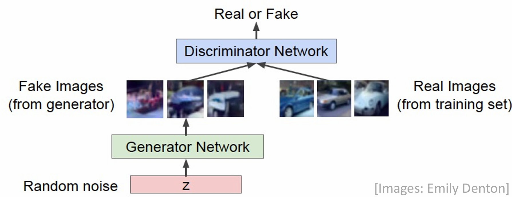
In these architectures, a generator network tries to fool the discriminator by generating real-looking images. In contrast, a discriminator network tries to distinguish between real and fake images. GANs don’t produce as good images as diffusion models, but the concept of adversarial learning is a crucial concept in many fields. The framework looks like this -

The objective function for a GAN is formulated as a mini-max game - the generator tries to maximize the loss function whereas the discriminator tries to reduce it.

\[L = \min_{\theta_g} \max_{\theta_d} [\mathbb E _{x \sim p_{data}} \log D_{\theta_d} (x) + \mathbb E_{z \sim p(z)} \log (1 - D(G_{\theta_g}(z)))]\]

The training is done alternately, performing gradient ascent on the generator and descent on the discriminator.

Object Detection

Simply put, the goal is identify objects in a given image. The evolution of algorithms for object detection is summarized as

• HoG + SVM - Sliding window mechanism for feature detection.

• Deformable Part Models (DPMs) -

• CNN - The vanilla approaches with CNNs proposed sliding a window across the image and use a classifier to determine if the window contains an object or not (one class is background). However, this is computationally expensive because we need to consider windows at several positions and scales. Following this, region proposals were designed to find blob-like regions in the image that could be an object. They do not consider the class and have a high rate of false positives which are filtered out in the next stages. Such class of methods are called multi-stage CNNs (RCNN, Fast-RCNN, Faster-RCNN) and are covered in detailed below. On the other hand, the sliding window approach has been optimised using anchor-boxes and this class of detectors are referred to as single-stage CNNs (YOLO series) which have been discussed in the next section. For more details, interested readers could also refer to my blog.

• Transformers - These methods are inspired from CNNs and have a transformer back-end. Examples include DETR and DINO discussed in later sections.

• Self-supervision

• Open vocabulary

Multi-stage CNNs

RCNN

For the region proposal network, an ImageNet pre-trained model (ResNet or like) is used. Since it has to be fine-tuned for detection, the last layer is modified to have 21 object classes (with background) instead of 1000 and is retrained for positive and negative regions in the image. The regions are then

FastRCNN

FasterRCNN

Uses a Region Proposal Network (RPN) after the last convolutional layer. The RPN is trained to produce region proposals directly without any need for external region proposals. After RPN, the RoI Pooling and an upstream classifier are used as regressors similar to FastRCNN.

Region Proposal Network

The network does the following -

• Slide a small window on the feature map

• A small network to do classification - object or no-object

• A regressor to give the bounding box

Anchors

Anchors are a set of reference positions on the feature map

3 dimensions with aspect ratio, 3 different scales of boxes,

Training

Non-Maximal Supression

Since, multiple anchor boxes can map to an object, we iteratively choose the highest scoring box among the predictions and supp ress the predictions that have high IoU with the currently chosen box.

Transformer based Architectures

DETR

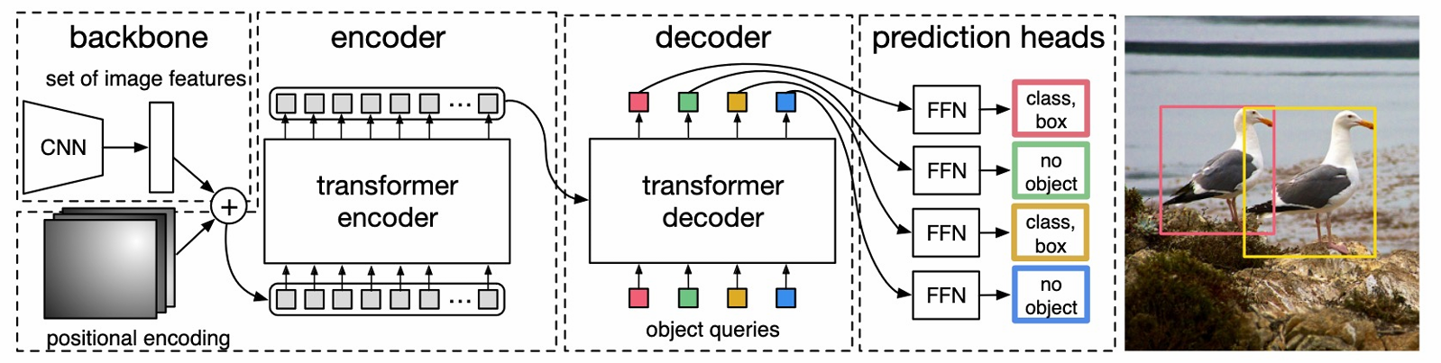
Faster R-CNN has many steps, handcrafted architecture and potentially non-differentiable steps. In contrast, DETR was proposed - an end-to-end transformer based architecture for object detection. The motivation was to capture all the human-designed optimization parts of the pipeline into one black-box using a transformer.

Why do we want such an end-to-end architecture? They are more flexible to diverse data, capturing large datasets, finetuning, etc.

In this architecture, a CNN backbone like ResNet extracts the features which are passed through the encoder to obtain latent representations. These are then used with a decoder along with object queries in the form of cross-attention to give bounding boxes as the output.

After obtaining the bounding boxes, the loss is appropriately calculated by matching the boxes to the correct labels. It is our task to assign a ground truth label to the predictions

Hungarian??

The decoder takes object queries as input,

500 epochs

encoder is segmented, decoder is just getting bounding boxes

DINO

lagging in scale variant objects.

contrastive loss acting for negative samples

YOLOX

Single Shot-Detectors

The motivation for these networks is to infer detections faster without much tradeoff in accuracy.

Anchor boxes

no ambiguous IoU

Hard negative mining

You Only Look Once (YOLO)

Divide into grids

anchor boxes in grid and class probability map

YOLO-X

No anchored mechanism - hyperparameter tuning, more predictions, less generalization (OOD fails)

Detection head decoupling, no anchor boxes, SimOTA

predict size and centers rather than top-left

mosaicing and mixing

Pyramid Feature Extractions

RFCN

Semantic Segmentation

The goal in this task is much more fine-tuned wherein we assign class pixel-wise. We want locally accurate boundaries as compared to finding bounding boxes in object detection. The approaches require global reasoning as well.

A naive approch would be to classify a pixel by considering the patch around the pixel in the image. This is very expensive computationally and does not capture any global information.

Another approach is to consider image resolution convolutions (purely convolutions with stride 1, no pooling) and maining the image resolution to produce the output. This still does not work quite well, and they also consume more memory.

Taking classification networks as the motications, some networks try pooling/striding to downsample the features. This architecture corresponds to the encoder part of the model, and the decoder then upsamples the image using transposed convolution, interpolation, unpooling to recover the spatial details in the original size. The convolutions can go deeper without occupying a lot of memory.

How do we upsample?

• Transposed convolution to upsample. The operation is shown below -

  ![Transpose Convolution for Up-Sampling Images

  Paperspace Blog](https://blog.paperspace.com/content/images/2020/07/conv.gif)

  However, the outputs are not very precise. Combine global and local information.

• U-Net

• Unpooling followed by convolutions (simpler implementation of transposed convolution)

  The max-unpooling operation does the following -

  Why is this better? Lesser memory

In all the architectures above, once you downsample the image, you lose a lot of spatial information and the network uses a significant amount of parameters learning the upsampling process to represent the final output. To help with this, we can do the following

• Predict at multiple scales and combine the predictions

• Dilated convolutions - These are used to increase the receptive field without downsampling the image too much -

  

  It’s multi-scale and also captures full-scale resolution. The idea of dilated convolution is very important in other tasks as well - It prevents the loss of spatial information in downsampling tasks. However, there are gridding artifacts and higher memory consumptions with Dilated networks.

  Degridding solutions

  • Add convolution layers at end of the network with progressively lower dilation

  • Remove skip connections in new layers, can propogate gridding artefacts because skip connections transfer high-frequency information.

• Skip-connections

DeepLab v3+

Segformer

Instance Segmentation

Mask RCNN

Predict eh

Panoptic Segmentation

Panoptic segmentation extends the idea of instance segmentation even further to segment objects beyond a fixed set of classes.

#

Universal Segmentation

Specialized architectures for semantic

MaskFormer

The architecture contains a strong CNN backbone for the encoder along with a query and pixel decoder. The query decoder essentially takes $n$ inputs to generate $n$ masks. The outputs from these layers are passed through an MLP to get binary masks for different classes.

Masked2Former

Uses a masked attention layer instead of cross-attention to provide faster convergence

Limitations

Needs to be trained on speicfic datasets, struggles with small objects and large inference time.

Hasn’t been extended to video segmentation and panoptic segmentation.

Mask DINO

Does both detection and segmentation. A Mask prediction branch along with box prediction in DINO.

Unified Denoising Training

Foundation Models

Models that have been trained on simple tasks which have good performance in the pipelines of other tasks for zero-shot transfer capabilities. Such models were first used in Natural Language Processing and using these in vision is typicalled hindered by unavailability of labeled data.

Segment Anything

A model developed by Meta with zero-shot segmentation capabilities. The task this model tries to solve is to allow for interactive and automatic use with zero-shot generatlization and re-use. The model allows for flexibile prompts with real-time usage and is ambiguity-aware. The model also has a data-engine which is used to generate data through the model.

Promptable segmentation

The model generates a valid mask for a given prompt (even if ambiguous) as input. How is the ambiguity resolved? Ambiguous cases arise when the mutiple objects lie on top of each other.

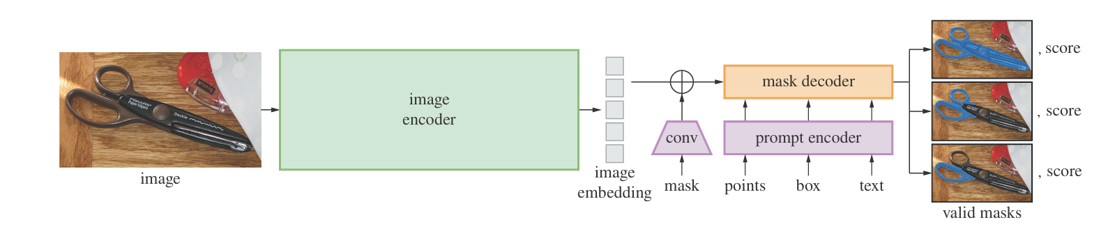
The image encoder is heavy - a pretrained ViT with masked autoencoder. The design choice for the masking involved masking around 75% of the patches. Unlike NLP tasks, vision tasks rely heavily on spatial information and neighbor patches can be reconstructed without much effort. Also, NLP tasks can get away with a simple MLP for decoders but vision taks require strong decoders.

The model allows for prompts using points, box or text. The decoder has self-attention on the primpts followed by cross-attention with image and MLP for non-linearity to get masks. The model also estimates the IoU to rank masks.

The emphasis of the model was also to make it universal. Since the encoder is heavy, the embeddings are precomputed after which the prompt encoder and mask decoder work quite fast.

Data Engine

There is no large-scale dataset available for training a segmentation model of this scale. Initially, the model has been trained iteratively on available datasets with several rounds of human correction. Following this, in the semi-automatic stage, the diversity of outputs (increasing ambiguity in overlapping objects) is improved by human refinement. Finally, in the fully automatic stage, prompting is introduced and masks with high IoU are preserved followed by NMS.

Zero-shot transfer capabilities

The idea is to fine-tune the model for specific tasks like edge-derection, object proposals and isntance segmentation.

Future Trajectory Prediction

This problem arises in many applications, particularly in autonomous driving. Given traffic participants and scene elements which are inter-dependent, we need to predict trajectories with scene awareness and multimodality. Humans are able to predict up to 10 seconds in highway scenes and plan their trajectory effectively whereas the SOTA models have a large gap in performance.

More concretely, the algorithm takes a video sequence as an input, and needs to predict probabilistic trajectories which are diverse, have 3D awareness, capture semantics interactions and focus on long-term rewards. There are many components in these solutions including 3D localization module, generative sampling modules, semantic scene modules and scene aware fusion modules with encoders and decoders.

#

Representation Framework

The past observed trajectories are represented by \(X = \{X_{i, t - l + 1}, \dots, X_{i, t}\}\) using we which we wish to predict future trajectory \(Y_i = \{Y_{i, t + 1}, \dots, Y_{i, t + \delta}\}\). The parameter \(\delta\) represents how far ahead we want to look in the future.

The sample generation module produces future hypotheses \hat Y, and then a ranking module assigns a reward to each hypothesis considering long-term rewards. Following this, the refinement step calculates the displacement \(\Delta Y_t\) for the selected trajectory.

Focusing on the sample generation module, the goal is to estimate posterior \(P(Y \vert X, I)\). Earlier, RNNs and other deterministic function maps from \(\{X, I\}\) to Y have been designed to address this. The problem with training in this approach is that the ground truth has a single future trajectory whereas the sampler predicts a distribution. How do we compare the two?

Principal Component Analysis

Principal component analysis (PCA) is a linear dimensionality reduction technique where data is linearly transformed onto a new coordinate system such that the directions (principal components) capturing the largest variation in the data can be easily identified. PCA works well when the data is near a linear manifold* in high dimensional spaces.

CAn we approximate PCA with a Network? Train a network with a bottleneck hidden layer, and try to make the output the same as the input. Without any activations, the neural network simply performs least-squares minimization which essentially is the PCA algorithm.

Adding non-linear activation functions would help the network map non-linear manifolds as well. This motivates for autoencoder networks.

Autoencoders

Network with a bottleneck layer that tries to reconstruct the input. The decoder can map latent vectors to images essentially helping us reconstruct images from a low-dimension. However, this is not truly generative yet since it learns a one-to-one mapping. An arbitrary latent vector can be far away from the learned latent space, and sampling new outputs is difficult.

### Variational Autoencoder

This network extends the idea in autoencoders and trains the network to learn a Gaussian distribution (parametrized by \(\mu, \sigma\)) for the latent space. After learning, say, the normal distribution, sampling is quite easy to generate new samples representative of the trianing dataset using the decoder.

To train this network, a distribution loss, like the KL-divergence is added in the latent space. But how do we backpropagate through random sampling? The reparametrization trick!

Conditional Variational Autoencoder

The encoder and decoder networks are now conditioned on the class variable.

Conditional Diffusion Models

Gradient of log, score function, conditioning at the cost of diversity - train a classifier and a diffusion model together in principle it’s fine. Potential issues - classifier can’t learn from noisy images and gradient of the classifier is not meaningful.

Classifier-Free Guidance

learn unconditional diffusion model \(p_\theta(x)\) and use the conditional model \(p_\theta(x \vert y)\) for some part of the training. this would not require any external classifier for training.

CTG++ - Language Guided Traffic Simulation via Scene-Level Diffusion

Testing autonomous agents in the real-world scenarios is expensive. Alternately, researchers aim to build good simulator that are realistic and can be controlled easily.

Why not RL-based methods? Designed long-term reward functions is difficult for such scenarios. The goal here is in a generation regime rather than problem solving. Also, the focus here is on controllability rather than realism. For realism, the methods would be more data-driven.

Trajectory Planning

Recent works have proposed diffusion-models for planning algorithms using classifier-guidance. Diffuser for example, is one such work where the authors generate state action pairs which are guided using a reward function to generate paths in a maze.

Traffic simulation methods

Early works for this task rrelied on rule-based algorithms which were highly controllable but not very realistic.

CTG

One of the first workd for diffusion models for planning and conditional guidance for control with STL-based loss. Howeber, it modelled each agent independently which caused issues.

CTG++ uses scene-level control

Problem Formulation

The state is given by the locations, speeds and angle of \(M\) agents whose past history and local semantic maps are given. We aim to learn a distribution of trajectories given this information.

The encoder represents the state action pairs in an embedded space on which temporal and cross attention on a diffusion based loss for training/

Inference

The model uses LLMs to generate code for guidance function.

Limitations and future work

CTG++ is able to generate more realistic example, but is still far-off from realism. There are no ablation studies or emperical evaluations with complicated scenarios. Also, the multi-agent modeling can be improved for scalability.

In conclusion, trajectory prediction requires generative models which are able to distinugish between feasible and infeasible trajectories. Variational Auto-Encoders have shown good performance for this task, and the current works aim to explore the scope of diffusion models in these tasks.

LeapFrog - Stochastic Trajectory Prediction

Similar to CTG++, this model aims to simulate real-world traffic scenarios. The authors aim for real-time predictions and better prediction accuracy. Leapfrog initializer skips over several steps of denoising and uses only few denoising steps to refine the distribtuion.

System Architecture

Leapfrog uses physics-inspired dynamics to reduce the number of steps required for the denoising process. The leapfrog initializer estimates mean trajectory for backbone of pericition, variance to control the prediction diversity and K samples simultaneously.

Limitations

The inference speed improved dramatically and achieves state of the art performance on the datasets. The model’s efficiency is higher for lower dimensional data and requires more work for scaling to higher dimensions.

Structure from Motion

The problem statement for structure from motion is - given a set of unordered or ordered set of images, estimate the relative positions of the cameras and recover the 3D structure of the world, typically as point clouds. In scenarios like autonomous driving, the images are ordered and the emphasis is on real-time performance.

Feature Detection

The first step involves identifying matching features across images to determine the camera movements. In unordered feature matching, the images to be compared are identified using vocabulary based retrieval methods to reduce the complexity from \(\mathcal O(n^2)\) to \(\log\) complexity.

In the canonical coordinate system, the camera axis passes through the origin, and the \(k\)-axis points away from the camera. The \(i\)-axis and \(j\)-axis are parallel to the image plane. The projection of 3D points in the pixel space involves a non-linear operation -

\[(x, y, z) \to (-d\frac{x}{z}, -d\frac{y}{z})\]

where \(d\) is the distance of the camera plane from the origin. For computational reasons, we want to convert these to a linear transformation. This is done via homogenous point representations -

\[\underbrace{(\frac{x}{w}, \frac{y}{w})}_\text{Euclidean} \to\underbrace{(x, y, w)}_\text{Homogenous}\]

Such representations are useful for ray marching operations. The camera transformation then becomes

\[\begin{bmatrix}-d & 0 & 0 & 0 \\ 0 & -d & 0 & 0 \\ 0 & 0 & 1 & 0 \end{bmatrix} \begin{bmatrix}x \\ y \\ z \\ 1\end{bmatrix} = \begin{bmatrix}-dx \\ -dy \\ z\end{bmatrix}\]

which represents \((-d\frac{x}{z}, -d\frac{y}{z})\) in Euclidean space. The matrix above can be decomposed as

\[\underbrace{\begin{bmatrix}-d & 0 & 0 \\ 0 & -d & 0 \\ 0 & 0 & 1 \end{bmatrix}}_{K}\underbrace{\begin{bmatrix}1 & 0 & 0 & 0 \\ 0 & 1 & 0 & 0 \\ 0 & 0 & 1 & 0 \end{bmatrix}}_\text{projection}\]

Here, we have considered a simple model for the camera intrinsics matrix \(K\) whose general form is

\[\begin{bmatrix}-d_x & s & c_x \\ 0 & -d_y & c_y \\ 0 & 0 & 1 \end{bmatrix}\]

where \(\alpha = \frac{d_x}{d_y}\) is the aspect ratio (1 unless pixels are not square), \(s\) is the skew, \(c_x, c_y\) represent the translation of the camera origin wrt world origin.

Coordinate Systems

We need to determine the transformations between the world and camera coordinate systems. Since camera is a rigid body, the transformation is represented by a translation and a rotation. Considering these, the projection matrix becomes

\[\Pi = K \begin{bmatrix} 1 & 0 & 0 & 0 \\ 0 & 1 & 0 & 0 \\ 0 & 0 & 1 & 0\end{bmatrix}\begin{bmatrix}R & 0 \\ 0 & 0 \end{bmatrix} \begin{bmatrix} T & - c \\ 0 & 0\end{bmatrix}\]

Problem Formulation

Given the projections \(\Pi_i X_i \sim P_{ii}\), we aim to minimize a non-linear least squares of the form \(G(R, T, X)\) -

\[G(X, R, T) = \sum_{i = 1}^m \sum_{j = 1}^n w_{ij} \cdot \left\|P(X_i, R_j, t_j) - \begin{bmatrix}u_{i, j} \\v_{i, j}\end{bmatrix} \right\|^2\]

This problem is called as Bundle Adjustment. Since this is an non-linear least squares, Levenberg-Marquardt is a popular choice to solve this. In theory, given enough number of points, we should get a unique solution. However, practically, we require a very good initialization to navigate the high-dimensional space. Also, outliers in the feature detection can deteriorate the performance of the model drastically.

Tricks for Real-world performance

Basically, we aim to make the feature detection very robust to remove all the possible outliers. Towards that, we note the following background

Fundamental Matrix

Given pixel coordinates \(x_1, x_2\) of a point \(x\) in two camera views, we define a fundamental matrix \(F\) such that \(x_1Fx_2 = 0\). The fundamental matrix is unique to the cameras and their relative configuration. It is given by

\[\begin{align*} F &= K_2^{-T} E K_1^{-1} \\ E &= [t]_{\times} R \end{align*}\]

where \(R\) and \([t]_\times\)represent the relative base transformations given by

\[[t]_X = \begin{bmatrix} 0 & -t_z & t_y \\ t_z & 0 & -t_x \\ -t_y & t_x & 0\end{bmatrix}\]

The matrix \(E\) is called as the essential matrix which has similar properties as the fundamental matrix and is also independent of the camera parameters.

The fundamental matrix is scale-invariant and has rank \(2\). Therefore, it has \(7\) degrees of freedom implying that we just need \(8\) correctly configured points (\(x\) and \(y\)) across the two pixel spaces to compute the fundamental matrix. We pose this problem as solving \(Af = 0\) - minimizing \(\|Af\|\) using SVD (to directly operate on the rank). This procedure is popularly known as the \(8\)-point algorithm. Furthermore, we can also use this to find the camera parameters by using more points.

The essential matrix can be derived from \(F\) using \(RQ\) decomposition to obtain skew-symmetric and orthogonal matrices \([t]_\times\) and \(R\). These matrices are what we were looking to determine - the relative configuration of the cameras with respect to each other. Now, triangulation can be used to locate \(x\) in the 3D space. However, this may not work since the projection lines may not intersect in 3D space.

To filter outliers, we will use the fundamental matrix as a model - it is a geometric property which all points have to abide by. However, the fundamental matrix itself is constructed from the detected features, which can be noisy. We need to design a robust method using heuristics to filter the outliers. We use a population-voting metric to choose the best model.

RANSAC

Suppose we are finding the best-fit line for a given set of points. For every pair of points, we determine the corresponding line and count the number of outliers for that particular line. The best model would then be the on which has the minimum number of outliers. This idea can be extended to any model, and it can be used to calculate the best fundamental matrix. The algorithm is as follows -

1. Randomly choose \(s\) samples - typically \(s\) is the minimum sample size to git a model (7 for a Fundamental matrix)
2. Fit a model to these samples
3. Count the number of inliers that approximately fit the models.
4. Repeat \(N\) times
5. Choose the model with the largest set of inliers.

How do we choose \(N\)? It depends on the ratio of outliers to the dataset size, the minimum number of samples \(s\) for the model and confidence score. We get

\[N = \frac{\log(1 - p)}{\log(1 - (1 - \epsilon)^s)}\]

Where \(\epsilon\) is the proportion of outliers and \(p\) is the confidence score.

Bundle Adjustment

Assuming we have a good \(R, t\) robust to outliers with the above methods, we can now solve the least-squares problem to determine the scene geometry.

Minimal Problems in computer Vision

Three—point absolute pose estimation

Assume the intrinsics of the camera are known. Determine the camera pose from given 3D-2D correspondences. Minimal case is 3 points: 6 degrees of freedom, 2 constraints per point \((u, v)\). Given \(p_1, p_2, p_3\) in world coordinates, find positions In camera coordinates. Equivalently, determine how to move camera such that corresponding 2D-3D points align.

Real-time SFM: Steady state

Suppose we have point-cloud and poses available at frame \(k\), find the pose in frame \(k + 1\).

Option 1

Find correspondences between consecutive frames, estimate the essential matrix and find \(R, t\). Keep repeating this as frames are read. 5 point estimation

Option 2

Estimate correspondences between point cloud and frame - 3 point absolute pose. Challenges - inliers calculations, which points to match. RANSAC maybe easier here. Option 1 is narrow baseline triangulation.

Drift Problem

Absolute scale is undeterminable. Why does scale matter? Noise and RANSAC. External measurements to fix this.

Loop Closure

Retrieval mechanism

Lighting

Unlike material properties and geometry, lighting is an external factor that is very complicated to infer. Lighting in a scene can. Be categorised as

• Local illumination - Li
• Global illumination

Shape

Normals Explicit representations Implicit representations - SDF

Inverse Rendering

PhySG

Geometry - SDF, Lighting - Environment map, Material (BRDF) Sphere Tracing! Monte Carlo integration for BRDFs - too slow. PhySG - spherical Gaussians

Neural Fields

The central question associated with neural fields is “what can be seen?”. That is, how can we measure what we see and how to model it for further computations? This question is important to not only the researchers in Computer Graphics but also in a field called Plenoptic Functions. It is basically the bundle of all light rays in a scene - a 5D function parametrized by position (\(x, y, z\)) and viewing direction (\(\theta, \phi\)). Neural Fields aim to approximate this function for a scene using Neural networks. Our core problem is that we have 2D slides and we need to estimate a 5D function. This problem is referred to as Image-based Rendering. It was taken into serious consideration in literature with the advent of the digital Michaelangelo project by Stanford, wherein researchers reconstructed the 3D models of all the sculptures in the Louvre museum. A closely related problem called “view synthesis” aims to generate images from views not present in the training data. In this problem, the 5D function is simplified to a 4D light field (rays passing through 3D space). Images are then captured from multiple view points, and novel view synthesis is done via interpolation with the closest rays. The earliest work in virtual reality by Sutherland in 1968, which talks about view synthesis and the ideas introduced in this paper are still relevant till date. The problem also gained interest in the graphics community - Chen et. al in SIGGRAPH 1993 talks about representing 3D models using images. However, researchers viewed view-synthesis as a small part of overall 3D scene understanding.

Perfect 3D understanding

Research then aimed to solve this problem rather than view synthesis. How is it different? In view syntheis, there is no information regarding the geometry of the scene itself. We want to infer the structure of the scene as well. So, how do we estimate the geometry of the scene?

Image-Depth Warping

As we have seen earlier, one of the first approaches for this problem was to perform feature detection and matching to triangulate points in 3D space. This core approach is being used in Depth from Stereo, multi-view stereo, 3D reconstruction, SLAM and so on. However, the output from these techniques is a point cloud which is sparse and contains “holes” which are not useful for the “structure of the scene”.

Surface reconstruction

Another subfield of graphics/vision tries to estimate the surface from these points clouds. There were methods using Local Gaussians, Local RBF functions, Local Signed Distance functions, etc. The famous approaches for this problem is Poisson surface reconstruction and Neural Signed Distance functions. In a way, Gaussian splatting is a surface reconstruction technique.

Space Carving

The underlying idea is motivatede from how humans create a sculpture - start out with a block, and carve/chip out regions that are not consistent with the camera viewpoints. However, this does not work well if there are not enough view points of the object (imaging back-projection problem in tomography).

Using Depth data

Suppose we have the depth information of each pixel as well - in such scenario, dealing with occlusions and “best-view planning” for 3D reconstruction becomes quite easy.

The slump

Between 2005 and 2014, there wasn’t much work done in the area of view synthesis, but many researchers focused on solving sub-problems in 3D scene understanding. There were papers for single-view depth estimation with a variety of diverse approaches. Along with these advances, the camera technologies also improved rapidly. Multi-array cameras were improved to hand-held cameras with much better resolution. The sensors to capture depth also improved - structured light was used in the past which did not work well in real-life scenarios. In contrast, we now have LIDARs to capture depth accurately and instantly. Given these advances, large-scale datasets came into place. KITTI dataset is one such famous dataset still being used as a benchmark for autonomous driving applications today. On the other front, GPUs improved exponentially, and the deep learning architectures grew better - ImageNet, Resnet, and other advances. With all these advances together, the focus on 3D reconstruction was on the rise again. Approaches using deep CNN networks, sparial transformer networks, etc were being applied to these problems. One key idea introduced in spatial transformer networks is differentiable samplers, which is an important property approaches aim to have now too.

3D understanding with Modern Tools

Since monocular reconstruction did not yield good results due to disocclusion problems, works focused on RGB\(\alpha\) planes wherein the depth was captured by multi-plane images. To get the image from a novel view point, alpha compositing is used to render the image. At this point, since we have perfect depth and color data from a viewpoint, we should be able to generate new views with ease. However, the novel views that can be generated are limited by single view data. Then, the idea of using multiple images of a scene started entering the literature.

What is the difference between depth map and MPI? Both capture the depth of the scene. Fast forward into the future, NeRFs started using multiplane images for each pixel rather than a single image.

Neural Radiance Fields

Alpha-composting is used to generate the value of each pixel in the rendering image, along with which, continuous volume rendering is done to represent the scene itself -

\[C_0 = \int C_t \sigma_t \exp\left(-\int \sigma_u du\right) dt\]

which is discretized as

\[C_0 = \sum_i C_i \alpha_i \prod_j (1 - \alpha_j)\]

Here, \(\sigma_t\) and \(\alpha\) are related to the transmittance/opacity of the pixel. The idea is that we shoot out a ray corresponding to a pixel in the camera image, sample points on the ray (ray-marching) to estimate their opacities and color. Neural networks are used to calculate the opacity for each spatial point and color value depending on the spatial location and viewing direction. The color depends on viewing direction because of BRDF functions that vary based on the viewing direction (image specular surfaces). Using the positions and viewing directions directly does not yield good results. Why? It is difficult to estimate high-frequency parameters required for images from these low-dimensional values. Neural networks tend to estimate low-frequency functions over high-frequency functions. To solve this, these coordinates are mapped to a high-dimensional space using positional encoding. This addition yields much superior results. Since the whole framework is completely differentiable, it is easy to find the optima minimizing the error across multiple camera views. NeRF was a very influential paper, enabling applications in new fields such as text-to-3D and it embodies the perfect combination of the right problem, at the right time, with the right people.

Mip-NeRF 360

The original paper has two major assumptions -

• Bounded scenes
• Front-facing scenes - camera views are limited to certain directions

The outputs from NeRF had a lot of aliasing issues when these assumptions are broken. Instead of assuming rays shooting out from the camera, Mip-Nerf shoots out conical frustrums with multivariate Gaussians to represent 3D volumes in the scenes. This solves the problem of front-facing scenes. To solve the problem of unbounded scenes, Mip-NeRF 360 uses “parameterization” to warp the points outside a certain radius using Kalman Filtering. Essentially, farther points are warped into a non-Euclidean space which is a tradeoff - for applications in SLAM and robotics, the geometry may be precisely needed which is sort of lost in such transformations. To speed up training in unbounded scenes, the authors proposed “distillation”, wherein sampling is done in a hierarchical manner to identify regions with higher opacities. These higher opacity regions are then used to estimate the color in the finer-sampled regions. To supervise the training of “density finding network”, the idea of distribution matching in multi-resolution histograms is used to formulate a loss function. Given limited number of camera, it is difficult to estimate all the parameters correctly - causing artefacts in the reconstructions. To solve this, the authors use a distortion regularizer to clump together points with higher densities. This acts as a prior to resolve some ambiguities in the scene.

Instant-NGP

Graphics Primitives

A form of representation for objects in the real-world. For example, an image is a graphics primitive that maps 2D pixels to RGB values.

So what is the motivation to have neural fields represent 3D volumes over voxels or point clouds? The latter are explicit representations which take up a lot of space!

NeRFs

We have seen that high-frequency encoding is used to effectively represent high-frequency features. This is a form of non-parametric encoding.

Parametric encodings on the other hand are more complicated, and can be used to learn feature vectors.

Multi-resolution hash-encoding

The scene is divided into multiple grids - the corners of each cube are hashed and stored in a hash table. For any point outside this lattice, we simply use a linear combination based on distances - this ensures continuity and differentiability.

What exactly is hashed? The high-dimensional vector embedding for each 3D point is stored. Furthermore, the authors implement a low-level CUDA kernel to realise fast matrix multiplications.

This implementation greatly reduces the training time and reduces the memory used. It takes days to train NeRFs, and with this the model could be trained in a couple of seconds.

Method Agnostic!

This idea is not only for NeRFs but can be used for other primitives like Gigapixel images, Neural SDFs, etc.

Weaknesses

• Rely on neural networks to resolve hash collisions - cause microstructure artifacts

• Hand-crafter hash function

• May not be robust to real world noise like flossy surfaces or motion blur.

3D Generative Models

Taking motivation from 2D generation, we use noise-sampling based approaches to build 3D scenes. While our 2D models are able to generate very high quality results, 3D models aren’t able to match these outputs. The first limitation is due to the unavailability of data (Objaverse-XL 10M vs LAION 5B). The dataset itself has very simple models, so it is difficult to build highly-detailed models.

Pretrained 2D Diffusion Models

How about Lifting Pretrained 2D Diffusion Models for 3D Generation? After the advent of NeRFs, this approach became feasible. The problem of creating a 3D model can be distilled to updated view-dependent 2D images!

To this end, people tried using diffusion models for the generative capabilities. An optimal denoiser should understand the image structure. What does this mean? The model needs to understand that there is a low-dimensional image-manifold in a high-dimensional space. The noising process takes the image out of this manifold whereas the denoising process tries to bring it back to this space - A projection function.

An important question arises here - How does the denoiser know which direction to project on? The models typically project to the weighted mean (Gaussian likelihood based) direction of the training samples. This is known as mean shifting - used widely in clustering methods.

How is this relevant to 3D generation? When we start with white noise, the initial direction would be towards the mean of all training samples. Elucidating the design space of Diffusion-Based Generative Models examines this property in detail. The mean-shift essentially generates more ‘likely’ samples.

Start out with a 3D blob, add Gaussian noise (to take it to the space where the diffusion model has been trained on) and then denoise it. The noise function used is

\[\partial \theta = \sum_i \mathbb E[w(\sigma) (\hat \epsilon_\phi (x_{c_i} + \sigma \epsilon) - \epsilon) \frac{\partial x_c}{\partial \theta}]\]

Alternately, DreamFusion: Text-to-3D using 2D Diffusion tries to optimize using a KL divergence loss function but further derivation shows that it is equivalent to the above loss function. This noise function is called as Score Distillation Sampling (SDS).

However, these still don’t yield good results. Here, researchers realised that unconditional distribution is much harder than conditional generation. Unconditional generation is still an open problem.

For conditional generation, text prompts are able to generate results with higher-fidelity. Authors in DreamFusion added some more tricks wherein they decomposed the scene into geometry, shading, and albedo to improve the results.

Mode-seeking

The score distillation sampling function (mean-shifting) has a mode-seeking behavior. This behavior is not necessarily good - it causes artefacts like saturated colors, lower diversity and fuzzy geometry. To alleviate these issues, there has been a new loss function crafted called variational score distillation.

Improvements

• Speed - Sampling speed can be improved using Gaussian Splatting

• Resolution - Resolution can be improved using Coarse-to-Fine refinement

Alternative Approaches

Multi-view 2D Generative Models

Fine-tune a 2D diffusion or any other generative model to generate multiple views of the same object. We pass in a single view of the object, and the generative model generates multiple views. This approach is explored in the paper Zero-1-to-3: Zero-shot One Image to 3D Object. Then, NeRF or Gaussian splatting can be used to create the 3D models. The problem becomes “Images-to-3D” which is a much more easier problem.

The recovered geometry may not have very good - the 2D models do not understand the geometry of the scene quite well.

Multi-view 2.5D Generative Models

Along with the RGB images, we could also estimate the normals to estimate the geometry better. This method is implemented in Wonder3D: Single Image to 3D using Cross-Domain Diffusion, and it obtains better results.

---

At this point, the Objaverse-XL dataset was released, and people tried to train image to 3D directly - LRM: Large Reconstruction Model for Single Image to 3D.

However, the issue with this approach is that since the dataset is object-centric and we want a more general model! Capturing such a general dataset is quite difficult.

An alternative idea could be to use videos as a dataset. Such an idea is explored in . Also, video generation is an achievable task with the current models - Sora.

People are still figuring out other ways to solve this general problem, and it is a very lucrative field - hundreds of papers in the past year!

Let us see some more papers which tried to address other issues in this problem.

#

Prolific Dreamer

As mentioned before, Google first released Dream Fusion for this problem. It used Imagen and Classifier-free guidance, but it did have the limitations mentioned before.

To improve on this performance, the authors of Prolific Dreamer modified the SDS Loss to something known as Variation Distillation Score - our goal is match the generated distribution with the distribution formed by multi-view images of a scene.

This is a difficult task as it is a sparse manifold in a complex high-dimensional space.

Do we have a metric to quantitatively analyse these models? T3 Bench is a benchmark score that checks the text-3D model alignment and the quality of the result itself.

ReconFusion

ZeroNVS is a modification over Zero-1-2-3 that does not require any pretraining on 3D models to generate models. However, this paper along with other approaches during this time required heavy pretrained models, with high computational requirements and scene specific fine-tuning. Along with these, they also had floater artifacts and inconsistencies in multi-view generation.

PixelNerf is one of the state-of-the-art 3D reconstruction papers that does not require dense training data because it relies on underlying pixel structure. The idea is to use this scene representation with latent diffusion models to address the limitations of the previous papers.

How do we train NeRF and Diffusion models simultaneously?

• We first have a reconstruction loss for the NeRF part wherein we sample a novel view and use some image similarity loss like L2 to optimize the network.

• Then, we have a sampling loss for the diffusion model that has LPIPS and a component for multi-view consistency

Interestingly, the authors choose DDIM for the diffusion model over stochastic sampling (probably helps with multi-view consistency).

Also, they use a trajectory based novel view sampling to further maintain consistency across views.

The resultant method is able to reconstruct a consistent 3D model even with inconsistent 2D views!

Vision and Language

The idea is to use an LLM agent to use language as a means to solve complex visual workflows. Along with human-curated high-level concepts, these can solve planet-scale problems. Robots can work on more general tasks - physically grounding them on images.

The main problem in realizing these models is aligning text and image concepts.

Pre-training Tasks: Generative

GPT uses causal modeling whereas BERT uses masked modeling. In the latter method, the words from the input data is masked out, and the model must predict the missing words. This allows global supervision allowing the model to look at both past and future data.

In context of images, we mask out some patches in the image and the model has to predict the remaining patches. This sort of an approach is displayed in Segment Anything Model (SAM).

However, some types of tasks may not support such a paradigm - text generation in a conversation. This is where causal modeling is used - the model is only allowed to look at the past data.

How do we do supervision in this case? It is similar to what we do in auto-regressive models for generating images and for generating text for images, it is similar to MLE.