Tensors

A scalar can be represented by a single component with zero basis vectors for each component.
A vector of 3 dimensions can be specified using three components and one basis vector for each component.
A stress matrix can be represented by nine components (we are considering 3 dimensions). That is two basis vectors for each component.

All of the above mathematical objects fall under a broad class of Tensors.

Tensors: In an $m$ dimensional space, a tensor of rank $n$ is a mathematical object that has $n$ indices, $m^n$ components and obeys certain transformation rules.

Generally, $m=3$ in real-life scenarios. $m=4$ is used while discussing relativity.

Rank of a tensor is defined as the number of basis vectors needed to fully specify a component of the tensor.

Transformation rules of tensors

A tensor is an object that transforms like a tensor
A tensor is an object that is an object that is invariant under a change of coordinate system with components that change according to a special set of mathematical formulae

In simpler terms, the actual tensor is invariant to a change in the coordinate systems. For example, the displacement vector pointing from $A$ to $B$ ( a $1$ rank tensor) does not change when coordinates change. The vector will still be pointing from $A$ to $B$. However, the way we represent the vector, i.e., the components changes.

Matrices $\neq$ Tensors

Matrices are a form of representation of rank-$2$ tensors. They are just an array of numbers. Although, Tensors require detailed specification and are invariant under change of coordinate systems.

Einstein Notation for Tensors

Both subscripts and superscripts are used for indices in tensors.

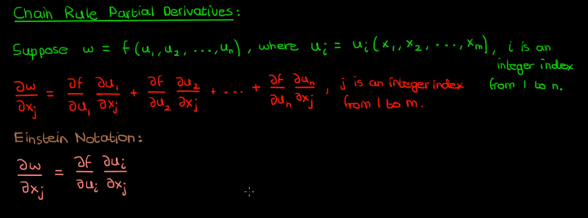
Any twice repeated index in a single term is summed over. Index $= 1, 2, \cdots , n$. Typically, $n = 3$

For example, $a_{ij}b_j = a_{i1} + a_{i2} + a_{i3}$

Here, $j$ is a dummy variable and $i$ is a free variable.

Dummy indices can be replaced, whereas free indices can’t be. A free index takes only one value in an expression.
No index may occur $3$ or more times in a given term.

$a_{ij}b_{ij} \checkmark$ $a_{ii}b_{ij} \pmb\times$ $a_{ij}b_{jj} \pmb\times$

We count subscripts and superscripts together. That is,

$a_j^j$ - $j$ is a dummy variable
In an equation involving Einstein notation, the free indices on both sides must match.

Brackets in Einstein Notation

Combine terms outside parentheses with each term inside parentheses separately.
From each of the combined terms, use the largest count of each index as the final count in the overall term.

Kronecker Delta

\[\delta_{ij} \equiv \delta_j^i \equiv \delta^{ij} \equiv \begin{cases}1 & i=j\\ 0 & i \neq j \end{cases}\]

Linear algebra of Tensors

For the following analysis, we shall be using the superscript notation to denote each element of a vector.

Rectangular coordinate system - A coordinate system ($x^i$) in $\mathbb R^n$ is rectangular if the distance between $2$ points $C(x^1, x^2, \cdots)$ and $D(x^1, x^2, \cdots)$ is given by : $\sqrt{\delta_{ij} \Delta x^i \Delta x^j}$

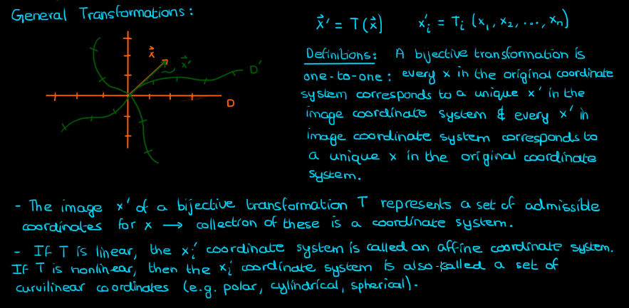
Curvilinear coordinates

$P$ is a point in a coordinate system ($x^i$) in $\mathbb R^n$ given by $P : (x^1,x^2, \cdots)$
$(\bar x^i)$ is another coordinate system in $\mathbb R^n$ such that the coordinates of $P$ in this system are $(\bar x^1,\bar x^2, \cdots)$
Suppose that $\bar x^i = \bar{x}^i(x^1, x^2, \cdots) : \mathcal{F}$. If the functions $\bar x^i(x^1, x^2, \cdots)$ are all real valued, have continuous $2$nd partial derivatives everywhere, and are all invertible then $\mathcal{F}$ is called a coordinate transformation.

The Jacobian is non-zero over a region $U$ in $\mathbb R^n$ iff the corresponding transformation $\mathcal{T}$ is locally bijective in that region $U$.

The Jacobian matrix of the inverse transformation $\mathcal{T}^{-1}$ is the inverse of the Jacobian matrix of $\mathcal{T}$

The above was taken from here

Recovering Joint Probability of Discrete Random Variables from Pairwise Marginals

Tensor Algebra

Canonical Polyadic Decomposition

If an $N$-way tensor $X \in \mathbb R^{I_1 \times I_2 \times \cdots \times I_N}$ has Canonical Polyadic rank $F$, it can be written as

$$ X(i_1, i_2, \cdots, i_N) = \sum_{f = 1}^{F} \lambda(f) \prod_{n = 1}^N A_n(i_n, f) $$

where $A_n \in \mathbb R^{I_n \times F}$ is called the mode-$n$ latent factor. In the above, $\lambda = [\lambda(1), \cdots, \lambda(F)]^T$ with $\|\lambda\|_0 = F$ is employed to ‘absorb’ the norms of columns.

In other words an $N$-way tensor $\mathcal{Z} \in \mathbb{R}^{I_1 \times I_2 \times \cdots \times I_N}$ representing the joint PMF of $N$ discrete RVs where $\mathcal{Z}(x_1, x_2, \cdots, x_N) = p(X_1 = x_1 , X_2 = x_2, \cdots, X_N = x_N)$, admits a CPD if it can be decomposed as a sum of $F$ rank-$1$ tensors. Denoting $a \otimes b$ as the outer-product (Kronecker Product) of two vectors, the CPD model is:

$$ \mathcal{Z} = \sum_{f = 1}^F \lambda(f)A_1(:,f)\otimes A_2(:,f) \otimes \cdots \otimes A_N(:,f) $$

Here, $F$ is the rank of the tensor.

Joint PMF Recovery: A Tensor Perspective

Any joint PMF admits a naive Bayes (NB) model representation; i.e., any joint PMF can be generated from a latent variable model with just one hidden variable. It follows that the joint PMF of $\{Z_n\}^N_{n=1}$ can always be decomposed as:

$$ Pr(i_1, i_2, \cdots, i_N) = \sum_{f = 1}^F Pr(f) \prod_{n=1}^N Pr(i_n | f) $$

where $Pr(f) := Pr(H = f)$ is the prior distribution of a latent variable $H$ and $Pr(i_n|f) := Pr(Z_n = z_n^{(i_n)} | H = f)$ are the conditional distributions.

Low Rank Tensor Recovery for Joint Probability Distribution