Miscellaneous

Supervised Machine Learning deals with the above 2 problems. Classification usually has discrete outputs while Regressions has continuous outputs.

Data preprocessing

Reading a csv using pandas

df = pd.read_scv(filepath)
# Creating dummy variables for Categorical columns
df = pd.get_dummies(data = df, columns = cat_cols)
from sklearn.preprocessing import LabelEncoder
#Encoding bool_cols
le = LabelEncoder()
for i in bool_cols :
    df[i] = le.fit_transform(df[i])

The preprocessing for numerical columns involves scaling them so that a change in one quantity is equal to another. The machines need to understand that just because some columns like ‘totalcharges’ have large values, it doesn’t mean that it plays a big part in predicting the outcome. To achieve this, we put all of our numerical columns into a same scale so that none of them are dominated by the other.

from sklearn.preprocessing import StandardScaler
#Scaling Numerical columns
std = StandardScaler()
scaled = std.fit_transform(df[num_cols])
scaled = pd.DataFrame(scaled,columns=num_cols)df.drop(columns = num_cols,axis = 1, inplace= True)
df = df.merge(scaled,left_index=True,right_index=True,how = "left")

Evaluation

For classification, the few common metrics we use to evaluate models are

• accuracy
• precision
• recall
• f1-score
• ROC curve, AUC

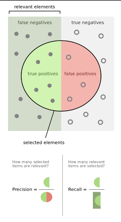
Precision and recall are defined as \(\text{Precision} = \frac{tp}{tp + fp} \\ \text Recall = \frac{tp}{tp + fn}\) Precision is defined as the percentage of your results which are relevant, Recall is defined as the percentage of relevant results correctly classified.

F1 Score

In general cases, there is a metric which harmonizes the precision and recall metric, which is the F1 Score. \(F = 2 \cdot \frac{\text{precision} \cdot \text{recall}}{\text{precision} + \text{recall}}\)

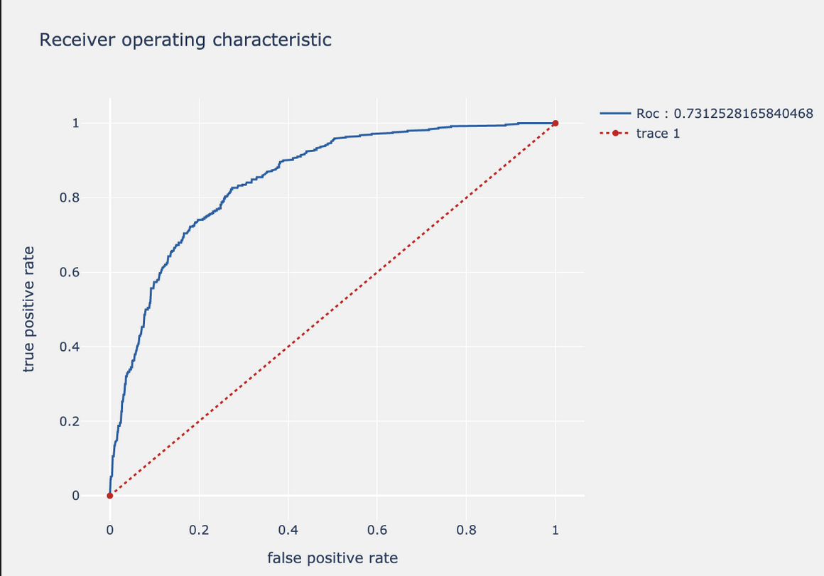
ROC curve and AUC

We can tweak the threshold of our models to improve the preferable metric. To visualise this change, we plot the effect of each threshold on the false and true positive rates. The curve looks like:

SSIM

Measures the similarity of images based on Luminance, contrast and Structural relations. Between 1 and -1. Often adjusted to [0, 1].

• Luminance is averaged across all pixels \(\mu_x = 1/N\sum_{i = 1}^N x_i \\ \text{Comparison is done using}\\ l(x, y) = \frac{2\mu_x\mu_y + C_1}{\mu_x^2 \mu_y^2 + C_1}\)

• Contrast is measured by taking the standard deviation of all pixel values. \(\sigma_x = \left(\frac{1}{N - 1}\sum_{i = 1}^N(x_1 - \mu_x)^2\right)^0.5 \\ \text{Comparison is done using}\\ l(x, y) = \frac{2\mu_x\mu_y + C_2}{\mu_x^2 \mu_y^2 + C_2}\)

• Structural comparison is done by using a consolidated formula which divides the normalised input signal with its standard deviation so that the result has unit standard deviation which allows for a more robust comparison. \(s(x, y) = \frac{\sigma_{xy} + C_3}{\sigma_x\sigma_y + C_3}\)

All of the above scores are multiplied.

Regression

Linear regression

Latent Semantic Analysis

LSA is a one of the most popular Natural Language Processing (NLP) techniques for trying to determine themes within text mathematically. It is an unsupervised learning technique that has two fundamental ideas

1. the distributional hypothesis, which states that words with similar meanings appear frequently together.
2. Singular value Decomposition (SVD)

In simple terms: LSA takes meaningful text documents and recreates them in n different parts where each part expresses a different way of looking at meaning in the text. If you imagine the text data as a an idea, there would be n different ways of looking at that idea, or n different ways of conceptualising the whole text. LSA reduces our table of data to a table of latent (hidden) concepts.

Suppose that we have some table of data, in this case text data, where each row is one document, and each column represents a term (which can be a word or a group of words, like “baker’s dozen” or “Downing Street”). This is the standard way to represent text data.

The product we’ll be getting out is the document-topic table (U) times the singular values (𝚺). This can be interpreted as the documents (all our news articles) along with how much they belong to each topic then weighted by the relative importance of each topic.

SVD is also used in model-based recommendation systems. It is very similar to Principal Component Analysis (PCA), but it operates better on sparse data than PCA does (and text data is almost always sparse). Whereas PCA performs decomposition on the correlation matrix of a dataset, SVD/LSA performs decomposition directly on the dataset as it is.

Tokenising and vectorising text data

Our models work on numbers, not string! So we tokenise the text (turning all documents into smaller observational entities — in this case words) and then turn them into numbers using Sklearn’s TF-IDF vectoriser.

The above part was not organised (clearly). I will try to summarise points in an organised way from here.

Data preprocessing

Turns out, this is a really important topic for Machine Learning in general. A real-world data generally contains noises, missing values, and maybe in an unusable format which cannot be directly used for machine learning models. Data preprocessing is required tasks for cleaning the data and making it suitable for a machine learning model which also increases the accuracy and efficiency of a machine learning model.

1. Get the dataset