Compressed Sensing

Recover a high dimensional vector $x$ with a very few non-zero values. Plethora of algorithms

Sensors and Measurements

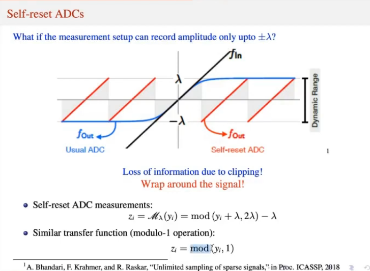
Sensors have Finite Dynamic Range
Loss of information due to clipping. One potential approach to fix this is to wrap around the signal.

This is where Modulo comes in.

Why can’t we scale the signal?

There is an inherent quantization step involved during measurements. Therefore, scaling down and scaling back up will have the same resolution.

Quantization error is proportional to the maximum value of the input signal.

Modulo Compressed Sensing

Typically, the real world sensors have a finite dynamic range. They have a clipping effect where the measurements become saturated once the values cross the range of the sensor. High dynamic range systems are affected by high quantization noise. To counter this problem, a new approach for measurements called self-reset analog to digital converters (SR-ADCs) have been proposed.

These sensors fold the amplitudes back into the dynamic range of the ADCs using the modulo arithmetic. However, these systems encounter loss due to the modulo operation. The transfer function of the SR_ADC with parameter $λ$ is given by

M_{λ} = 2 λ ([[\frac{t}{2 λ} + \frac{1}{2}]] - \frac{1}{2})

Here, $[[t]] ≜ t = ⌊ t ⌋$ . Now, we need to consider how we shall sample the values. A sampling theory called unlimited sampling framework was developed which provides sufficient conditions on the sampling rate for guaranteeing the recovery of band-limited signals from the folded samples. SR-ADC is applied individually to multiple linear measurements of the images, and is termed as modulo compressed sensing.

Note. The measured values may lie outside the dynamic range due to sensor noise.

Let us concretely define the problem. Let $x \in R^{N}$ denote an $s$ -sparse vector ( $| | x | |_{0} \leq s$ ) with $s < \frac{N}{2}$ . We obtain $m$ projections of $x$ as follows:

z_{i} = [[⟨ a_{i}, x ⟩]], i = 1, 2, \dots, m

Usually, $m \leq N$ in the compressed sensing paradigm. Stacking these projections, we get

z = [[y]] = [[A x]]

The non-linearity introduced by the modulo operation along with the undetermined compressive measurements could lead to an indeterminate system.

$P_{0}$ : Any real valued vector $y \in R^{m}$ can be uniquely decomposed as $y = z + v$ where $z \in [0, 1)^{m}$ and $v \in Z^{m}$ denote the fractional and integral part of $y$ respectively. The following optimization problem is defined as $P_{0}$

\arg min_{x, v} ‖ x ‖_{0} subject to A x = z + v; v \in Z^{m}

Notice that $v$ is the integral part and not $z$ , which may be confusing.

The optimization equation does not oblige $z$ to belong to $[0, 1)^{m}$ . In fact, this condition is implicitly taken care when we impose minimality over $z$ .

The $‖ w_{0} ‖$ condition comes due to the sparsity of $w$ .

Any $s^{'}$ sparse solution to $P_{0}$ such that $s^{'} \leq s$ is also $s$ sparse.

Identifiability

Lemma. Any vector $x$ satisfying $‖ x ‖_{0} \leq s < \frac{N}{2}$ is a unique solution to the optimization problem $P_{0}$ iff any $2 s$ columns of matrix $A$ are linearly independent of all $v \in Z^{m}$

Proof.

( $\to$ ) Suppose a set of $2 s$ columns of $A$ , say $S$ , are not linearly independent. That is,

A y = w \in Z^{m} where y \in R^{n} has support S

Consider a vector $x$ defined from $y$ whose support is the first $s$ columns of $S$ . Similarly, define $x_{1}$ whose support is the remaining $s$ columns of $S$ . Let $A x = z + v$ where $z \in (0, 1)^{m}$ and $v \in Z^{m}$ . We have

A x_{1} = A y - A x = w - (z + v)

Therefore, $- x_{1}$ and $x$ are both solutions of $P_{0}$ . This is a contradiction. This proves sufficiency.

( $\leftarrow$ ) Let $z \in (0, 1)^{m}$ and $v, v_{1} \in Z^{m}$ such that $A x = z + v$ and $A x_{1} = z + v_{1}$ where $‖ x ‖_{0}, ‖ x_{1} ‖_{0} \leq s$ . Now, the size of the support of $x - x_{1}$ is at most $2 s$ . Consequently,

A (x - x_{1}) = v - v_{1} \in Z^{m}

This is a contradiction as any $2 s$ columns of $A$ are linearly independent of all $v \in Z^{m}$ . This proves necessity.

Corollary. Any vector $x$ satisfying $‖ x ‖_{0} \geq \frac{N}{2}$ is a unique solutions to $P_{0}$ iff columns of $A$ are linearly independent. Consequently, the minimum number of measurements required for unique recovery is m = $N + 1$ (not $N$ , see below)

Conditions for recovery

Signals in spacial domain

To compare the modulo-CS problem to the standard CS problem, we state the two necessary conditions for modulo-CS recovery.

The following two conditions are necessary for recovering any vector $x$ satisfying $‖ x ‖_{0} \leq s$ as a unique solution to $P_{0}$ :

$m \geq 2 s + 1$ , and
Any $2 s$ columns of $A$ are linearly independent.

$m = 2 s$ is necessary and sufficient for unique sparse recovery in the standard CS setup. We now show $m = 2 s + 1$ measurements is sufficient for unique recovery.

Theorem. For any $N \geq 2 s + 1$ , there exists a matrix $A \in R^{m \times N}$ with $m = 2 s + 1$ rows such that every $s$ -sparse $x \in R^{N}$ can be uniquely recovered from its modulo measurements $z = [[A x]]$

Proof. We define the following

$V = {v | v \in Z^{m}}$ denotes the countably infinite set of all integer vectors.
$G = {T | T \subset [N], | T | = 2 s}$ denotes the set of all index sets on $[N]$ whose cardinality is $2 s$ .

Let $A$ be a matrix for which at least one $s$ - sparse vector $x$ cannot be recovered from $z = [[A x]]$ via $(P_{0})$ . Our aim is to show the set of all such matrices is of Lebesgue measure zero.

For a given $u \in V$ and $S \in G$ , construct $B (u, S) = [\begin{matrix} u & A_{S} \end{matrix}]$ . If $d e t (B (u, S))$ equals $0$ , then $A$ is not linearly independent of $Z^{m}$ . This function is a non-zero polynomial of the entries of $A_{s}$ , and therefore the set of matrices which satisfy this condition have Lebesgue measure zero.

Now, consider $\cup_{S \in G} \cup_{u \in V} {A | d e t (B (u, S)) = 0}$ , This set is of Lebesgue measure zero (why?). Therefore, any matrix $A$ chosen outside this set will ensure that any $s$ -sparse vector $x$ can be recovered from $y = [[A x]]$ .

If the entries of $A$ are drawn independently from any continuous distribution, $A$ lies outside the set of Lebesgue measure 0 described in the above theorem.
Integer matrices cannot be used as candidate measurement matrices for modulo CS (why?)

Signals in Temporal domain

Unlimited Sampling Theorem - A band-limited signal can be recovered from modulo samples provided that a certain sampling density criterion is satisfied. This criterion must be independent of the ADC threshold.

Theorem. Let $f (t)$ be a function with no frequencies higher than $Ω$ (rad/s), then a sufficient condition for recovery of $f (t)$ from its modulo samples $y_{k} = M_{λ} (f (t)), t = k T, k \in Z$ is,

$T \leq \frac{1}{2 Ω e}$

The above guarantees the recovery of the signal. Now, we discuss the conditions for unique recovery. There is a one-to-one mapping between a band-limited function and its modulo samples provided that the sampling rate is higher than the Nyquist Rate, $T < π / Ω$ .

Theorem. Let $f (t)$ be a finite-energy function with no frequencies higher than $Ω$ (rad/s). Then the function $f (t)$ is uniquely determined by its modulo samples $y_{k} = M_{λ} (f (t_{k}))$ taken on grid $t = k T_{ϵ}, k \in Z$ where

$0 < T_{ϵ} < \frac{π}{Ω + ϵ}, ϵ > 0$

Convex Relaxation

Replacing the $l_{0}$ -norm in $P_{0}$ with the $l_{1}$ -norm, we obtain the optimization problem:

P_{1} : \arg min_{x, v} ‖ x ‖_{1} subject to A x = z + v; v \in Z^{m}

Integer Range Space Property

A matrix $A$ is said to satisfy the IRSP of order $s$ if, for all sets $S \subset [N]$ with $| S | \leq s$ ,

‖ u_{S} ‖_{1} < ‖ u_{S^{c}} ‖_{1}

holds for every $u \in R^{N}$ with $A u = v \in Z^{m}$ .

Theorem. Every $s$ -sparse $x$ is the unique solution of $(P_{1})$ iff the matrix $A$ satisfies the IRSP of order s.

Proof.

( $\to$ ) Consider a fixed index set $S$ with $| S | \leq s$ , and suppose that every $x$ supported on $S$ is a unique minimizer of $(P_{1})$ . Then, for any $u$ such that $A u = v \in Z^{m}$ , the vector $u_{S}$ is the unique minimizer of $(P_{1})$ . But, $A (u_{S} + u_{S^{c}}) \in Z^{m}$ . This means that $u_{S^{c}}$ is also a solution of $(P_{1})$ for $[[A u_{S}]] = y$ . Consequently, (we are talking about $l_{1}$ -norm not $l_{0}$ -norm)

‖ u_{S} ‖_{1} < ‖ u_{S^{c}} ‖_{1}

( $\leftarrow$ ) Suppose IRSP holds with respect to the set $S$ . Consider $x$ supported on $S$ and another vector $x^{1}$ that result in the same modulo measurements with respect to $A$ . Let $u = x - x^{1}$ , the vector $A u \in Z^{m}$ . Due to the IRSP,

‖ u_{S} ‖_{1} < ‖ u_{S^{c}} ‖_{1}

Hence,

\begin{aligned} (1) & ‖ x ‖_{1} & \leq ‖ x - x_{S}^{1} ‖_{1} + ‖ x_{S}^{1} ‖_{1} \\ (2) & = ‖ u_{S} ‖_{1} + ‖ x_{S}^{1} ‖_{1} \\ (3) & < ‖ u_{S^{c}} ‖_{1} + ‖ x_{S}^{1} ‖_{1} \\ (4) & = ‖ - x_{S^{c}}^{1} ‖_{1} + ‖ x_{S}^{1} ‖_{1} = ‖ x^{1} ‖_{1} \end{aligned}

Thus proving uniqueness.

Mixed Linear Integer Program (MILP)

The $l_{1}$ -norm can be re-written as a linear function using two positive vectors $x^{+}$ and $x^{-}$ , where $x = x^{+} - x^{-}$ . This leads to the MILP formulation

min_{x^{+}, x^{-}, v} 1^{T} (x^{+} + x^{-}) subject to [\begin{matrix} A & - A & - I \end{matrix}] [\begin{matrix} x^{+} \\ x^{-} \\ v \end{matrix}] = z; v \in Z^{m}; x^{+}, x^{-} \geq 0

This is efficiently solved using branch-and-bound algorithm.

Appendix - Lebesgue Measure

Lebesgue measure is an extension of the classical notions of length, area and volume to more complicated sets. Given an open set $S \equiv \sum_{k} (a_{k}, b_{k})$ containing disjoint intervals, the Lebesgue measure is defined by

μ_{L} (S) = \sum_{k} (b_{k} - a_{k})

Refer to this document for more details regarding this topic.

Let $A \subseteq R$ . $A$ is said to be of measure zero if for any $ϵ > 0$ , there exists a sequence of open intervals $(I_{n})_{n \in N}$ such that,

A \subseteq ⋃_{n = 1}^{\infty} I_{n} and \sum_{n = 1}^{\infty} l (I_{n}) < ϵ

where, $l ((a, b)) = b - a$ . For example, $Q$ is of measure zero.

Modulo Compressed Sensing

Compressed Sensing

Sensors and Measurements

Why can’t we scale the signal?

Modulo Compressed Sensing

Identifiability

Conditions for recovery

Signals in spacial domain

Signals in Temporal domain

Convex Relaxation

Integer Range Space Property

Mixed Linear Integer Program (MILP)

Appendix - Lebesgue Measure

Enjoy Reading This Article?

Talk to my AI