Lecture 1

Numerical Analysis is the study of various methods

• to solve
  • differential equations,
  • systems of linear equations,
  • \(f(x) = \alpha\).
• to approximate functions and
• to study the corresponding errors.

Example. \(e = \lim_{n \to \inf} (1 + 1/n)^n)\). How do we approximate \(e\) to an arbitrary accuracy? Since, the \(exp\) function is infinitely many times differentiable, we can approximate the function using Taylor’s theorem to any degree of precision we want.

Using this, we get

where \(c\) is some real number between 0 and 1. Here, the error term at the \(n\)-th approximation is the term \(e^c/(n + 1)!\). We know that \(e^c\) is less than 3 so we can compute \(n\) where the error term is less than the prescribed error!

For example, suppose we want the error to be less than \(10^{-10}\), then we use \(e^c/(n + 1)! < 10^{-10}\).

Note. The last term is not the error in our approximation! We are choosing \(e^c = 3\) for no particular reason. It can be any value greater than the true value of \(e^c\). For instance, we can take \(e^c = 1000\) too. If we want our calculated value \(e\) value to be precise till the 10th decimal, then we ensure that \(1000/(n + 1)! < 10^{-10}\) by tuning \(n\) appropriately.

Aspects of numerical analysis

• The theory behind the calculation, and
• The computation.

Some calculators have a loss of information due to limits in precision. This is due to the round-off error. We need to be able to detect and deal with such cases.

Lecture 2

Finite digit arithmetic

When we do arithmetic, we allow for infinitely many digits. However, in the computational world, each representable number has only a fixed and finite number of digits. In most cases, the machine arithmetic is satisfactory, but at times problems arise because of this discrepancy. The error that is produced due to this issue is called the round-off error.

A 64-bit representation is used for a real number. The first bit is a sign indicator, denoted by s. This is followed by an 11-bit exponent, c, called the characteristic, and a 52-bit binary fraction, f, called the mantissa. To ensure that numbers with small magnitude are equally representable, 1023 is subtracted from the characteristic, so the range of the exponent is actually from -1023 to 1024.

Thus, the system gives a floating-point number of the form

Since 52 binary digits correspond to between 16 and 17 decimal digits, we can assume that a number represented in this system is accurate till the 16th decimal.

Can’t a single number be represented in many ways through this representation? Think about 1 for instance.

The smallest positive number that can be represented is with \(s = 0, c = 1, f = 0\), so it is

Numbers occurring in calculations that have a magnitude less than this number result in underflow and are generally set to 0.

The largest positive number is

Numbers above this would result in an overflow.

Floating-point representation

We will use numbers of the form

with \(1 \leq d_1 \leq 9\). There are two ways to get the floating-point representations \(fl(p)\) of a positive number \(p\)

• Chopping. We simply chop off the \(d_{k + 1}, d_{k + 2}, \dots\) and write \(0.d_1d_2\dots d_k \times 10^n\)
• Rounding. We add \(5 \times 10^{n - (k + 1)}\) to the number and then chop the result to obtain \(0.\delta_1\delta_2\dots \delta_k \times 10^n\)

Errors

This approximate way of writing numbers is bound to create errors. If \(p\) is a real number and if \(p^*\) is its approximation then the absolute error is \(\|p - p ^*\|\) while the relative error is \(\|p - p ^*\|/p\) whenever \(p \neq 0\). Relative error is more meaningful as it takes into account the size of the number \(p\).

Note. Relative error can be negative as we take the value of \(p\) in the denominator!

Significant digits

We say that the number \(p^*\) approximates \(p\) to \(t\) significant digits if \(t\) is the largest non-negative integer for which

Finite Digit Arithmetic

The arithmetic in machines in defined by the following -

Lecture 3

Major sources of errors

One of the major sources of errors is cancellation of two nearly equal numbers. Suppose we have

In the above set of equations, the difference \(x \ominus y\) has \(k - p\) digits of significance compared to the \(k\) digits of significance of \(x\) and \(y\). The number of significant digits have reduced which leads to errors in further calculations.

Another way the errors creep in is when we divide by number of small magnitude or multiply by numbers of large magnitude. This is because the error gets multiplied by a factor which increases its absolute value.

Consider the expression \(-b \pm \sqrt{b^2 - 4ac}/2a\). By default, we consider positive square roots. Here, if \(b^2\) is large compared to \(4ac\) then the machine is likely to treat \(4ac\) as zero. How do we get around this error? Rationalization

​ Notice what happened here. Previously, the roots would have become zero because \(4ac\) could have been approximated as zero. However, this does not happen after rationalization! Also, do note that this won’t work when \(b<0\) as we are considering positive square roots. If \(b<0\), we can use the formula without rationalization. Think about the other root using such cases. Thus, the cancellation error can come in two major ways:

• when we cancel two nearly equal numbers, and
• when we subtract a small number from a big number

Errors propagate

Once an error is introduced in a calculation, any further operation is likely to contain the same or a higher error.

Can we avoid errors?

Errors are inevitable in finite arithmetic. There are some measures that we can take to try to avoid errors, or minimize them. For example, a general degree 3 polynomial can be written as a nested polynomial.

Computations done using this form will typically have a smaller error as the number of operations has reduced (from 5 to 3). Now, we are done with the first theme of our course - Machine arithmetic.

Lecture 4

Roots of equations

The zeros of a function can give us a lot of information regarding the function. Why specifically zero? Division is in general more difficult to implement in comparison to multiplication. Division is implemented via the solution to roots of an equation in computers. There are other reasons such as eigenvalue decomposition. We shall see all of this later in the course.

Theorem. Intermediate Value Theorem. If \(f: [a, b] \to \mathbb R\) is a continuous function with \(f(a)\cdot f(b) < 0\) then there is a \(c \in [a, b]\) such that \(f(x) = 0\).

Bisection method

The bisection method is implemented using the above theorem. To begin, we set \(a_1 = a\) and \(b_1 = b\), and let \(p_1\) be the midpoint of \([a, b]\);

• If \(f(p_1) = 0\), then we are done
• If \(f(p_1)f(a_1)>0\), then the subinterval \([p_1, b_1]\) contains a root of \(f\), we then set \(a_2 = p_1\) and \(b_2 = b_1\)
• If \(f(p_1)f(b_1)>0\), then the subinterval \([a_1, p_1]\) contains a root of \(f\), we then set \(a_2 = a_1\) and \(b_2 = p_1\)

We continue this process until we obtain the root. Each iteration reduces the size of the interval by half. Therefore, it is beneficial to choose a small interval in the beginning. The sequence of \(\{p_i\}\) is a Cauchy sequence. IT may happen that none of the \(p_i\) is a root. For instance, the root may be an irrational number and \(a_1, b_1\) may be rational numbers. There are three criteria to decide to stop the bisection process.

• \(\|f(p_n)\| < \epsilon\) - not very good because it may take a long time to achieve it, or that it may be achieved easily and yet \(p_n\) is significantly many steps away from a root of \(f\)
• \(\|p_n - p_{n-1}\| <\epsilon\) is not good because it does not take the function \(f\) into account. While \(p_n\) and \(p_{n-1}\) may be close enough but the actual root may still be many steps away.
• \(p_n \neq 0 \text{ and } \frac{\|p_n - p_{n-1}\|}{\|p_n\|} < \epsilon\) looks enticing as it mimics the relative error but again it does not take \(f\) into account.

The bisection method has significant drawbacks - It is relatively slow to converge, and a good intermediate approximation might be inadvertently discarded. However, the method has the important property that is always converges to a solution.

Lecture 5

Fixed points and roots

A fixed point of \(f : [a,b] \to \mathbb R\) is \(p \in [a,b]\) such that \(f(p) = p\). Finding a fixed point of the function \(f\) is equivalent to finding the root of the function \(g(x) = f(x) - x\). We can create many such functions which give fixed points of \(f\) on solving for the roots of the function.

Theorem. Fixed Point Theorem. If \(f: [a,b] \to [a,b]\) is continuous then \(f\) has a fixed point. If, in addition, \(f’(x)\) exists on \((a, b)\) and \(\vert f’(x)\vert \leq k < 1\) for all \(x \in (a, b)\) then \(f\) has a unique fixed point in \([a, b]\).

The hypothesis is sufficient but not necessary!

Fixed point iteration

We start with a continuous \(f: [a,b] \to [a,b]\). Take any initial approximation \(p_0 \in [a,b]\) and generate a sequence \(p_n = f(p_{n - 1})\). If the sequence \(\{p_n\}\) converges to \(p \in [a, b]\) then

This method is called the fixed point iteration method. It’s convergence is not guaranteed.

For instance, consider the roots of the equation \(x^3 + 4x^2 - 10 = 0\). The following functions can be used to find the roots using the fixed points.

The results using different \(g\)’s in the Fixed Point Iteration method are surprising. The first two functions diverge, and the last one converges. This problem is because the hypothesis of the FPT does not hold in the first two functions. While the derivative \(g’(x)\) fails to satisfy in the FPT, a closer look tells us that it is enough to work on the interval \([1, 1.5]\) where the function \(g_3\) is strictly decreasing.

So now we have the question - How can we find a fixed point problem that produces a sequence that reliably and rapidly converges to a solution to a given root-finding problem?

Lecture 6

Newton-Raphson method

This is a particular fixed point iteration method. Assume that \(f: [a, b] \to \mathbb R\) is twice differentiable. Let \(p \in [a, b]\) be a solution of the equation \(f(x) = 0\). If \(p_0\) is another point in \([a, b]\) then Taylor’s theorem gives

\[\begin{align} 0 &= f(p) \\ &= f(p_0) + (p - p_0)f'(p_0) + \frac{(p - p_0)^2}{2}f''(\xi) \end{align}\]

for some \(\xi\) between \(p\) and \(p_0\). We assume that \(\vert p - p_0 \vert\) is very small. Therefore, \(0 \approx f(p_0) + (p - p_0)f’(p_0)\). This sets the stage for the Newton-Raphson method, which starts with an initial approximation \(p_0\) and generate the sequence \(\{p_n\}\) by

\[p_n = p_{n - 1} - \frac{f(p_{n - 1})}{f'(p_{n - 1})}\]

What is the geometric interpretation of this method? It approximates successive tangents. The Newton-Raphson method is evidently better than the fixed point iteration method. However, it is important to note that \(\vert p - p_0 \vert\) is need to be small so the third term in the Taylor’s polynomial can be dropped.

Theorem. Let \(f: [a, b] \to \mathbb R\) be twice differentiable. If \(p \in (a, b)\) is such that \(f(p) = 0\) and \(f’(p) \neq 0\), then there exists a \(\delta > 0\) such that for any \(p_0 \in [p - \delta, p + \delta]\), the Newton-Raphson method generates a sequence \(\{p_n\}\) converging to \(p\).

This theorem is seldom applied in practice, as it does not tell us how to determine the constant \(\delta\). In a practical application, an initial approximation is selected and successive approximations are generated by the method. These will generally either converge quickly to the root, or it will be clear that convergence is unlikely.

Lecture 7

Problems with the Newton-Raphson method

We have

\[p_n = p_{n - 1} - \frac{f(p_{n - 1})}{f'(p_{n - 1})}\]

One major problem with this is that we need to compute the value of \(f’\) at each step. Typically, \(f'\) is far more difficult to compute and needs more arithmetic operations to calculate than \(f\).

Secant method

This method is a slight variation to NR to circumvent the above problem. By definition,

\[f'(a) = \lim_{x \to a} \frac{f(a) - f(x)}{a - x}\]

If we assume that \(p_{n - 2}\) is reasonable close to \(p_{n - 1}\) then

\[f'(p_{n - 1}) \approx \frac{f(p_{n - 1}) - f(p_{n - 2})}{p_{n - 1} - p_{n - 2}}\]

This adjustment is called as the secant method. The geometric interpretation is that we use successive secants instead of tangents. Note that we can use the values of \(f(p_{n - 2})\) from the previous calculations to prevent redundant steps. We need two initial guesses in this method.

Secant method is efficient in comparison to Newton-Raphson as it requires only a single calculation in each iteration whereas NR requires 2 calculations in each step.

The method of false position

The NR or the Secant method may give successive approximations which are on one side of the root. That is \(f(p_{n - 1}) \cdot f(p_n)\) need not be negative. We can modify this by taking the pair of approximations which are on both sides of the root. This gives the regula falso method or the method of false position.

We choose initial approximations \(p_0\) and \(p_1\) with \(f(p_0)\cdot f(p_1) < 0\). We then use Secant method for successive updates. If in any iteration, we have \(f(p_{n - 1})\cdot f(p_n) > 0\), then we replace \(p_{n - 1}\) by \(p_{n - 2}\).

The added requirement of the regula falsi method results in more calculations than the Secant method.

Comparison of all the root finding methods

• The bisection method guarantees a sequence converging to the root but it is a slow method.
• The other methods are sure to work, once the sequence is convergent. The convergence typically depends on the initial approximations being very close to the root.
• Therefore, in general, bisection method is used to get the initial guess, and then NR or the Secant method is used to get the exact root.

Lecture 8

We are reaching the end of the equations in one variable theme.

Order of convergence

Let \(\{p_n\}\) be a sequence that converges to \(p\) with \(p_n \neq p\) for any \(n\). If there are positive constants \(\lambda\) and \(\alpha\) such that

\[\lim_n \frac{\vert p_{n + 1} - p \vert}{\vert p_n - p \vert^\alpha} = \lambda\]

then the order of convergence of \(\{p_n\}\) to \(p\) is \(\alpha\) with asymptomatic error \(\lambda\). An iterative technique of the form \(p_n = g(p_{n - 1})\) is said to be of order \(\alpha\) if the sequence \(\{p_n\}\) converges to the solution \(p = g(p)\) with order \(\alpha\).

In general, a sequence with a high order of convergence converges more rapidly than a sequence with a lower order. The asymptotic constant affects the speed of convergence but not to the extent of the order.

Two cases of order are given special attention

• If \(\alpha = 1\) and \(\lambda < 1\), the sequence is linearly convergent.
• If \(\alpha = 2\), the sequence is quadratically convergent.

Order of convergence of fixed point iteration method?

Consider the fixed point iteration \(p_{n + 1} = f(p_n)\). The Mean Value Theorem gives

\[\begin{align} p_{n + 1} - p &= f(p_n) - f(p) \\ &= f'(\xi_n)(p_n - p) \end{align}\]

where \(\xi_n\) lies between \(p_n\) and \(p\), hence \(\lim_n\xi_n = p\). Therefore,

\[\lim_n \frac{\vert p_{n + 1} - p \vert}{\vert p_n - p \vert} = \lim_n \vert f'(\xi_n)\vert = \vert f'(p)\vert\]

The convergence of a fixed point iteration method is thus linear if \(f’(p) \neq 0\) and \(f’(p) < 1\).

We need to have \(f’(p) = 0\) for a higher order of convergence.

why?

Theorem. Let \(p\) be a solution of the equation \(x = f(x)\). Let \(f’(p) = 0\) and \(f’'\) be continuous with \(\vert f''(x) \vert < M\) nearby \(p\). Then there exists a \(\delta > 0\) such that, for \(p_0 \in [p - \delta, p + \delta]\), the sequence defined \(p_n = f(p_{n - 1})\) converges at least quadratically to \(p\). Moreover, for sufficiently large values of \(n\)

\[\vert p_{n+1} - p \vert < \frac{M}{2}\vert p_n - p \vert^2\]

For quadratically convergent fixed point methods, we should search for functions whose derivatives are zero at the fixed point. If we have the root-finding problem for \(g(x) = 0\), then the easiest way to construct a fixed-point problem would be

\[\begin{align} f(x) &= x - \phi(x)g(x)\\ f'(x) &= 1 - \phi'(x)g(x) - \phi(x)g'(x) \\ 0 &= f'(p) = 1 - \phi(p)g'(p) \\ & \implies \phi(p) = {g'(p)}^{-1} \end{align}\]

where \(\phi\) is a differentiable function, to be chosen later. Therefore, define \(phi(x) = {g’(x)}^{-1}\) which gives

\[p_{n + 1} = f(p_n) = p_n - \frac{g(p_n)}{g'(p_n)}\]

This is the Newton-Raphson method! We have assumed that \(g’(p) \neq 0\) in the above analysis. The NR/Secant method will not work if this assumption fails.

Multiplicity of a zero

Let \(g: [a, b] \to \mathbb R\) be a function and let \(p \in [a, b]\) be a zero of \(g\). We say that \(p\) is a zero of multiplicity \(m\) of \(g\) if for \(x \neq p\), we can write \(g(x) = (x - p)^mq(x)\) with \(\lim_{x \to p}q(x) \neq 0\).

Whenever \(g\) has a simple zero (\(m = 1\)) at \(p\), then the NR method works well for \(g\). However, NR does not give a quadratic convergence if the order of the zero is more than 1.

Lecture 9

Note. \(n\)-digit arithmetic deals with \(n\) significant digits and not \(n\) places after the decimal.

Order of the fixed point iteration method

Summarizing the last lecture we have

• If we have a function \(g(x)\) whose roots are to be found, we can convert it to a fixed point problem by appropriately constructing a \(f(x)\).
• If we construct \(f(x)\) such that it’s derivative is non-zero at the root, then the fixed point iteration method is linear.
• Otherwise, if the derivative is zero, then the fixed point iteration method is quadratic or higher. For example, we constructed such a \(f(x)\) which mirrored the Newton-Raphson method.
• In the Newton-Raphson method itself, if the root is a simple zero of \(g\), the method has quadratic convergence. However, if it is not a simple zero if \(g\) then the method may not have a quadratic convergence.

Can we modify NR to overcome the limitation of multiplicity of the zero?

Modified Newton-Raphson

For a given \(g(x)\), we define a function \(\mu\)

\[\mu(x) = \frac{g(x)}{g'(x)}\]

If \(x = p\) is a xero of \(g\) with multiplicity \(m\), we have

\[\mu(x) = (x - p)\frac{q(x)}{mq(x) + (x - p)q'(x)}\]

Notice that \(x = p\) is a simple root of \(\mu\). Further, assume \(g, q\) are continuous. Then, if \(g(x)\) has no other zero in a neighborhood of \(x = p\) then \(\mu(x)\) will also not have any other zero in that neighborhood. We can now apply Newton-Raphson method to \(\mu(x)\).

The fixed point iteration is given by

\[\begin{align} f(x) &= x - \frac{\mu(x)}{\mu'(x)} \\ &= x - \frac{g(x)/g'(x)}{(g'(x)^2 - g(xg''(x)))/g'(x)^2} \\ &= x - \frac{g(x)g'(x)}{g'(x)^2 - g(x)g''(x)} \end{align}\]

This iteration will converge to \(p\) with at least the quadratic order of convergence. The only theoretical drawback with this method is that we now need to compute \(g’’(x)\) at each step. Computationally, the denominator of the formula involves cancelling two nearly equal terms (\(x = p\) is a root of both \(g, g’\)).

Note that if \(x = p\) is a simple zero, the modified Newton-Raphson still bodes well. It’s just that there are a lot more calculations in the modified NR method.

An other methods?

There are many methods other than the 4 we considered so far. Suppose that \(\{p_n\}\) converges to \(p\) linearly. For large enough \(n\), we have \((p_{n + 1} - p)^2 \approx (p_n - p)(p_{n + 2} - p)\) which further gives

\[p \approx p_n - \frac{(p_{n + 1} - p_n)^2}{p_{n + 2} - 2p_{n + 1} + p_n} = \hat p_n\]

This is called Aitken’s \(\mathbf{\Delta^2}\)-method of accelerating convergence. So, if we have a sequence \(\{p_n\}\) converging to \(p\) linearly, we can come up with an alternate sequence \(\{\hat p_n\}\) using the original sequence that converges faster.

This brings us to the end of the second theme of our course - Equations in one variable.

Lecture 10

We begin the third theme of our course - Interpolation

Polynomials are very well studied functions. They have the form \(P(x) = a_nx^n + \cdots + a_1x + a_0\). Given any continuous function \(f: [a, b] \to \mathbb R\), there exists a polynomial that is as close to the given function as desired. In other words, we can construct a polynomial which exactly matches the function in a finite interval. This is known as Weierstrass approximation theorem. Another reason to prefer polynomials is that the derivatives of polynomials are also polynomials.

Taylor polynomials

We can consider the polynomials formed by Taylor’s theorem. However, these polynomials approximate the function only at a single point. The advantage of using these polynomials is that the error between the function and the polynomial can be determined accurately. For ordinary computational purposes it is more efficient to use methods that include information at various points.

Lagrange interpolating polynomials

Let \(f\) be a function with \(f(x_0) = y_0\). Is there a polynomial \(P(x)\) with \(P(x_0) = y_0\).

The simplest case is \(P(x) = y_0\). If we have two points \(x_0\) and \(x_1\), then we can have \(P(x) = y_0\frac{x - x_1}{x_0 - x_1} + y_1\frac{x - x_0}{x_1 - x_0}\) . We can generalize this for more number of points.

Let \(x_0, x_1, \dots, x_n\) be distinct \((n + 1)\)-points and let \(f\) be a function with \(f(x_i) = y_i, \forall i \in [n]\). We want to find a polynomial \(P\) that equals \(f\) at these points. To do this, we first solve \(n + 1\) special problems, where \(y_i = \delta_{i, n + 1}\). We find polynomials \(L_{n, i}\) with

\[L_{n, i}(x_j) = \delta_{i, j} = \cases{0 & i $\neq$ j \\ 1 & i = j}\]

For a fixed \(i\), \(L_{n, i}(x_j) = 0\) for \(j \neq i\). So \((x - x_j)\) divides \(L_{n, i}(x)\) for each \(j \neq i\). Since the points \(x_i\) are all distinct, we have that the product of all such \((x - x_j)\)‘s divides \(L_{n, i}(x)\). We define \(L_{n, i}(x)\) as

\[L_{n, i}(x) = \frac{(x - x_0)\dots(x - x_{i - 1})(x - x_{i + 1})\dots (x - x_n)}{(x_i - x_0)\dots(x_i - x_{i - 1})(x_i - x_{i + 1})\dots(x_i - x_n)}\]

then \(L_{n, i}(x_j) = \delta_{i, j}\). Now, \(P\) can be constructed as

\[P(x) = y_0L_{n, 0}(x) + \dots + y_nL_{n, n}(x)\]

The validity of this polynomial can be checked easily.

Lecture 11

What if you take a linear function and use \(n >2\) points for Lagrange interpolation? Will the final function be linear? It should be.

For example, in class we considered \(f(1) = 1\) and \(f(2) = 1\). These values gave a constant polynomial.

In general, for \((n + 1)\)-points, the interpolating polynomial will have degree at most \(n\).

Uniqueness of the interpolating polynomial

For a given set of \((n + 1)\) points, we can have infinitely many polynomials which interpolate it. However, there exists a unique polynomial with degree \(\mathbf {\leq n}\). This result follows from the well-known theorem -

Theorem. A polynomial of degree \(n\) has at most \(n\) distinct zeroes.

Corollary. A polynomial with degree \(\leq n\) with \((n + 1)\) zeroes is the zero polynomial.

Error of the interpolating polynomial

Theorem. Let \(f:[a,b] \to \mathbb R\) be \((n + 1)\)-times continuously differentiable. Let \(P(x)\) be the polynomial interpolating \(f\) at distinct \((n + 1)\) points \(x_0, x_1, \dots, x_n \in [a, b]\). Then, for each \(x \in [a, b]\), there exists \(\xi(x) \in (a, b)\) with

\[f(x) = P(x) + \frac{f^{(n + 1)}(\xi(x))}{(n + 1)!}(x - x_0)(x - x_1)\cdots (x - x_n)\]

How? Intuition?

Using the above theorem, we can calculate the maximum possible value of the absolute error in an interval.

Note. While checking for extreme values in an interval, do not forget to check the value of the function at the edge of the interval!

Lecture 12

Note. The value of \(\xi(x)\) for the error calculation depends on the point \(x\) at which error is being calculated.

Practical difficulties with Lagrange Polynomials

To use the error form, we need some information about \(f\) in order to find its derivative. However, this is often not the case. Also, the computations of the lower degree interpolating polynomials does not quite help the computations of the higher degree ones. We would like to find a method that helps in computing the interpolating polynomials cumulatively.

Cumulative calculation of interpolating polynomials

Let us assume that \(f\) is given on distinct nodes \(x_0, x_1, \dots, x_n\). Now, the constant polynomial for the node \(x_0\) will be \(P_0(x) = f(x_0)\) and that for the node \(x_1\) will be \(Q_0(x) = f(x_1)\). Using Lagrange interpolation, we have

\[\begin{align} P_1(x) &= \frac{x - x_1}{x_0 - x_1}f(x_0) + \frac{x - x_0}{x_1 - x_0}f(x_1) \\ &= \frac{(x - x_1)P_0(x) - (x - x_0)Q_0(x)}{(x_0 - x_1)} \end{align}\]

Can we generalize this? Let us try to construct the quadratic polynomial. Now, suppose we have \(P_1(x)\) and $Q_1(x)$. The quadratic polynomial for the nodes \(x_0, x_1, x_2\) is given by,

\[\begin{align} P_2(x) &= \frac{x - x_2}{x_0 - x_2}\left[\frac{x - x_1}{x_0 - x_1}f(x_0) + \frac{x - x_0}{x_1 - x_0}f(x_1)\right] \\ - &\frac{x - x_0}{x_0 - x_2}\left[\frac{x - x_2}{x_1 - x_2}f(x_1) + \frac{x - x_1}{x_2 - x_1}f(x_2)\right] \\ \\ &= \frac{(x - x_2)P_1(x) - (x - x_0)Q_1(x)}{x_0 - x_2} \end{align}\]

We shall see the general formula in the next lecture.

Lecture 13

Before we move on to the general formula, let us take the previous calculations one step further. Suppose we had to calculate the cubic polynomial in terms of the quadratic polynomials. The tedious way to do this is to expand each formula and substitute. We also have an easy way to do this. Recall the ‘unique polynomial’ theorem from last week. If we guess the formula of the cubic polynomial using induction, then all we have to do is check the value of the function at the 4 points which define it. If the value matches, then it is the polynomial we are looking for due to uniqueness.

Neville’s formula

Let \(f\) be defined on \(\{x_0, x_1, \dots, x_n\}\). Choose two distinct nodes \(x_i\) and \(x_j\). Let \(Q_i\) be the polynomial interpolating \(f\) on all nodes except \(x_i\), and let \(Q_j\) be the one interpolating \(f\) on all nodes except \(x_j\). If \(P\) denotes the polynomial interpolating \(f\) on all notes then

\[P(x) = \frac{(x - x_j)Q_j(x) - (x - x_i)Q_i(x)}{x_i - x_j}\]

In Neville’s formula we can get the interpolating for higher degree from any two polynomials for two subsets of nodes which are obtained by removing a single node. Through such cumulative calculations, we can calculate the interpolating polynomials up to a certain degree until we get the required accuracy. Neville’s method gives the values of the interpolating polynomials at a specific point, without having to compute the polynomials themselves.

Divided Differences

Given the function \(f\) on distinct \((n + 1)\) nodes, there is a unique polynomial \(P_n\) interpolating \(f\) on these nodes. We define \(f[x_0, \dots, x_n]\) to be the coefficient of \(x^n\) in \(P_n\). Now, it follows readily that the value of \(f[x_0, \dots, x_n]\) does not depend on the ordering of the nodes \(x_i\). Now, we shall try to get a recurrence formula for the coefficients \(f[x_0, \dots, x_n]\).

Let \(P_{n - 1}\) and \(Q_{n - 1}\) be the polynomials interpolating \(f\) on the nodes \(x_0, \dots, x_{n - 1}\) and \(x_1, \dots, x_n\) respectively. We can get \(P_n\) from these two polynomials using Neville’s method. The coefficient of \(x^n\) in \(P_n\) is then

\[\frac{\text{coefficient of } x^{n - 1} \text{ in } Q_{n - 1} - \text{coefficient of } x^{n - 1} \text{ in } P_{n - 1}}{x_n - x_0} \\ = \frac{f[x_1, \dots, x_n] - f[x_0, \dots, x_{n - 1}]}{x_n - x_0}\]

Also note that for \(i < n, P_n(x_i) = P_{n - 1}(x_i)\). That is, \(P_n - P_{n - 1} = \alpha(x - x_0)\dots (x - x_{n - 1})\) where \(\alpha\) is a real number. Hence, \(f[x_0, \dots, x_n] = \alpha\) and we have

\[P_n = P_{n - 1} + (x - x_0)\dots (x - x_{n - 1})f[x_0, \dots, x_n]\]

This formula is known as Newton’s finite differences formula.

Lecture 14

We have

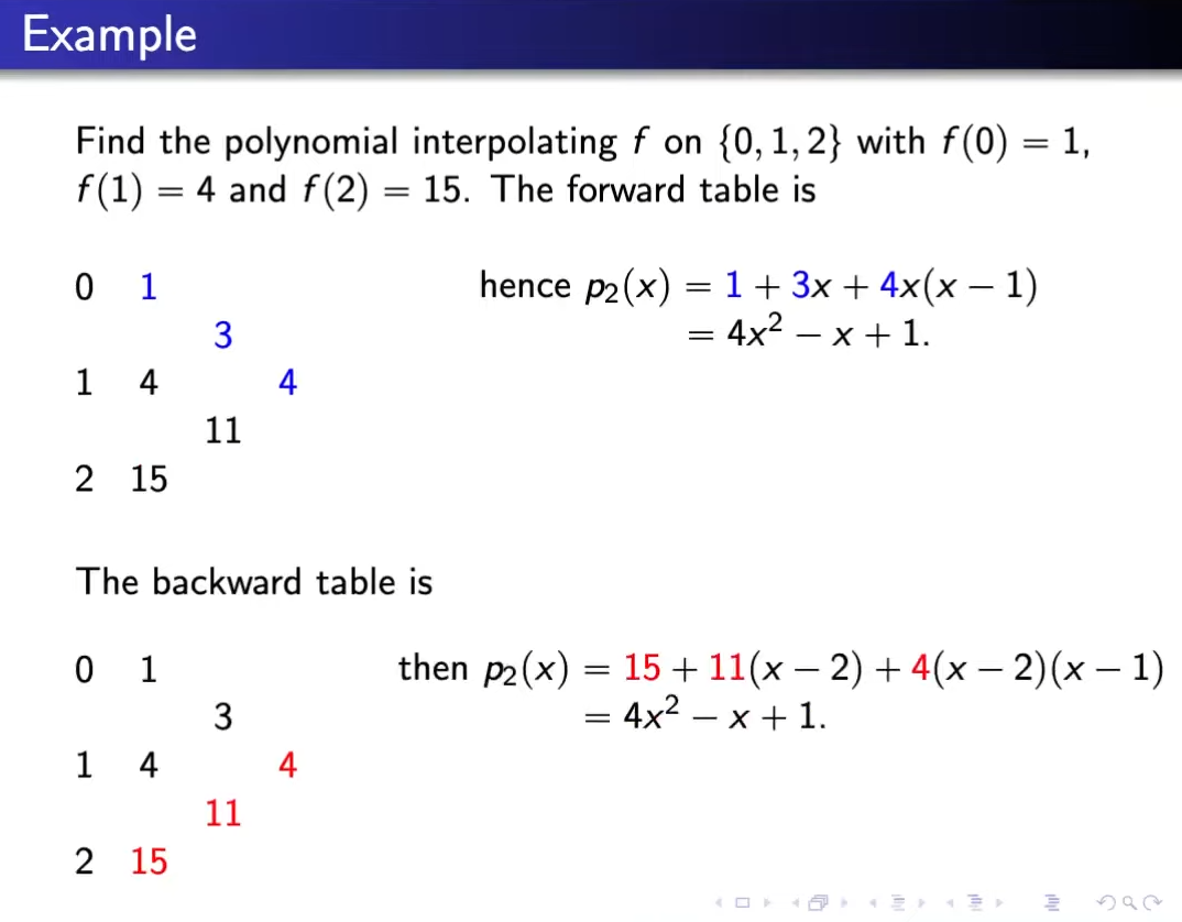
\[P_n - P_{n - 1} = f[x_0, \dots, x_n](x - x_0)\dots (x - x_{n - 1}) \\ \\ f[x_0, \dots, x_n] = \frac{f[x_1, \dots, x_n] - f[x_0, \dots, x_{n - 1}]}{x_n - x_0}\]

Since the order of the nodes does not matter, we can traverse the recursion in a forward/backward manner. The forward formula is given by,

\[P_n(x) = f(x_0) + f[x_0, x_1](x - x_0) + f[x_0, x_1, x_2](x - x_0)(x - x_1) + \\ \cdots + f[x_0, x_1, \dots, x_n](x - x_0)\cdots (x - x_{n - 1})\]

The backward formula simply replaces \(i\) by \(n - i\) for \(i \in [0, \dots, n]\). For clarity, look at the following example.

Nested form of the interpolating polynomial

\[P_n(x) = f(x_0) + (x - x_0)\big[f[x_0, x_1] + (x - x_1)[f[x_0, x_1, x_2] + \\ \cdots + (x - x_{n - 1})f[x_0, \dots, x_n]\big]\]

Neste form of the interpolating polynomial is useful for computing the polynomials \(P_n\) effectively.

Divided differences as a function

We now give a definition of the divided differences when some of the nodes may be equal to each other. By the Mean Value Theorem, \(f[x_0, x_1] = f’(\xi)\) for some \(\xi\) between \(x_0\) and \(x_1\). In fact, we also have the following theorem,

Theorem. If \(f\) is \(n\)-times continuously differentiable on \([a, b]\) then

\[f[x_0, \dots, x_n] = \frac{f^{(n)}(\xi)}{n!}\]

for some \(\xi \in [a, b]\).

Since \(f[x_0, x_1] = f'(\xi)\) for some \(\xi\) between \(x_0\) and \(x_1\), we define \(f[x_0, x_0] = f’(x_0) = \lim_{x_1 \to x_0}f[x_0, x_1]\). Similarly, we define \(f[x_0, \dots, x_n]\) in a similar way using limits. For instance,

\[f[x_0, x_1, x_0] = \frac{f[x_0, x_1]- f'(x_0)}{x_1 - x_0}\\ f[x_0, x_0, x_0] = f^{(2)}(x_0)/2\]

We have thus defined \(f[x_0, \dots, x_n]\) in general. Now, by letting the last \(x_n\) as variable \(x\), we get a function of x: \(f[x_0, \dots, x_{n - 1}, x]\). This function is continuous.

\[f[x_0, x] = \begin{cases} \frac{f(x) - f(x_0)}{x - x_0} & x \neq x_0 \\ f'(x_0) & x = x_0 \end{cases}\]

MA214 post-midsem notes

• Composite numerical integration - Newton-Cotes doesn’t work for large intervals. Therefore, we divide the interval into sub-parts. We are essentially doing a spline sorta thing instead of a higher degree polynomial. \(\begin{align} \int_a^b f(x)dx &= \sum_{j = 1}^{n/2} \left\{\frac{h}{3}[f(x_{2j - 2} + 4f(x_{2j - 1} + f(x_{2j}] - \frac{h^5}{90}f^{(4)}(\xi_j)\right\} \\ &= \frac{h}{3}\left[f(a) + 2\sum_{j = 1}^{n/2 - 1}f(x_{2j}) + 4\sum_{j = 1}^{n/2}f(x_{2j - 1}) + f(b)\right] - \frac{b - a}{180}h^4f^{(4)}(\mu) \end{align}\)

• Error in composite trapezoidal rule is \(\frac{b - a}{12}h^2f''(\mu)\), and in composite Simpson’s rule is \(\frac{b - a}{180}h^4f''(\mu)\).

• The round-off error does not depend on the number of calculations in the composite methods. We get \(e(h) \leq hn\epsilon = (b - a)\epsilon\) Therefore, integration is stable.

• Adaptive Quadrature method - \(S(a, b) - \frac{h^5}{90}f^{(4)}(\xi) \approx S(a, \frac{a+ b}{2}) + S(\frac{a + b}{2}, b) - \frac{1}{16}\frac{h^5}{90}f^{(4)}(\xi')\) We will assume \(f^{(4)}(\xi) \approx f^{(4)}(\xi’)\). Using this assumption, we get that composite Simpson’s rule with \(n = 2\) is 15 times better than normal Simpson’s rule. If one of the subintervals has error more than \(\epsilon/2\), then we divide it even further.

  Check this properly!

• Gaussian Quadrature method -

  Choose points for interval in an optimal way and not equally spaced. We choose \(x_i\) and \(c_i\) to minimise the error in \(\int_a^bf(x)dx \approx \sum_{i = 1}^nc_if(x_i)\) There are \(2n\) parameters, then the largest class of polynomials is the set of polynomials with degree \(2n - 1\) for the approximation to be exact.

  Note. Work with special cases of polynomials like \(1, x, x^2, \dots\) to get the values of the coefficients easily. (because all polynomials in the set must satisfy the approximation)

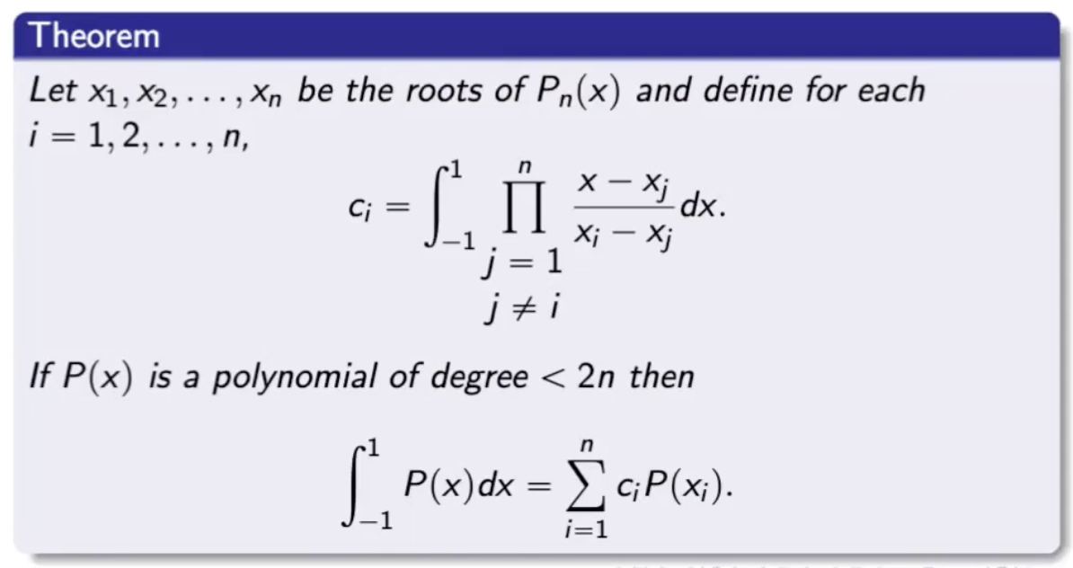
  Legendre polynomials - There exist polynomials \(\{P_n(x)\}\) for \(n = 0, 1, \dots\)satisfying

  • \(P_n(x)\) is a monic polynomials
  • \(\int_{-1}^1P(x)P_n(x) = 0\) whenever the degree of \(P(x)\) is less than \(n\).

  For example, \(P_0(x) = 1, P_1(x) = x\). \(P_2\) can be computed from \(P_0\) and \(P_1\) as \(\int P_0P_2\) and \(\int P_1P_2\) are 0.

  

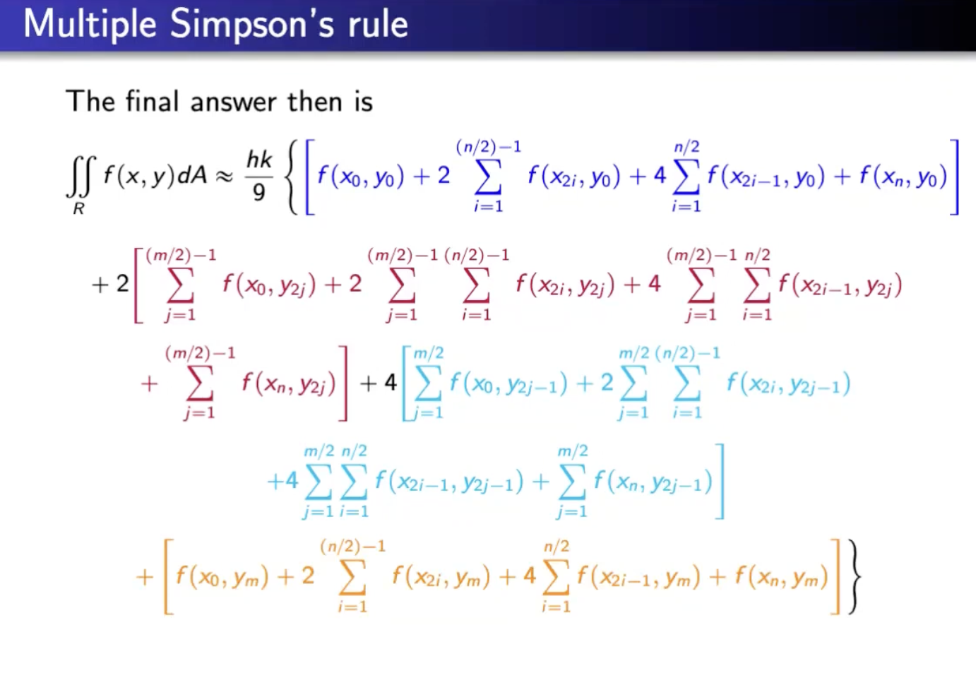
• Multidimensional integrals - Composite trapezoidal rule has square of the number of function evaluations required for a single integral (for 2D).

  

  See if problems to be practiced here.

• Improper integrals - Function is unbounded or the interval is unbounded. We will deal with functions where the function is unbounded on the left end.

• Aside. \(a^b\) is defined as \(\exp(b \log a)\) in the complex domain. \(\log\) is not defined as the inverse of \(\exp\) as \(\exp\) is neither surjective (doesn’t take the value 0) nor injective (periodic in \(\mathbb C\)). \(\exp\) is defined by the power series and so is \(\log\). The solution set of \(z\) for \(e^z = w\) where \(z, w \in \mathbb C\) is given by \(\{\log |w| + \iota(\arg w + 2\pi k) : k \in \mathbb Z\}\)

  If \(f(x) = \frac{g(x)}{(x - a)^p}\) where \(0 < p< 1\) and \(g: [a,b] \to \mathbb R\) is continuous then the improper integral \(\int_a^b f(x)dx\) exists. Assume \(g\) is 5-times continuously differentiable. We can estimate the integral of \(f(x)\) using the following

  • Get \(P_4(x)\) which is the 4th degree Taylor’s polynomial of \(g\).
  • Get the exact value of \(\int_a^b P_4(x)/(x - a)^p\).
  • Get the value of the difference by defining the value at \(z = a\) as \(0\) using composite Simpson’s rule.

  Why can’t we do Simpson’s on everything? That would lead to a similar thing. Think. Also, we require 4 times continuously differentiable for Simpson’s

  The other type of improper integral involves infinite limits of integration. The basic integral is of the type \(\int_a^\infty 1/x^p dx\) for \(p > 1\). Then, we substitute \(x = 1/t\) and proceed.

• Ordinary Differential Equations We shall develop numerical methods to get solutions to ODEs at a given point. Then, we can use interpolation to get an approximate continuous solution.

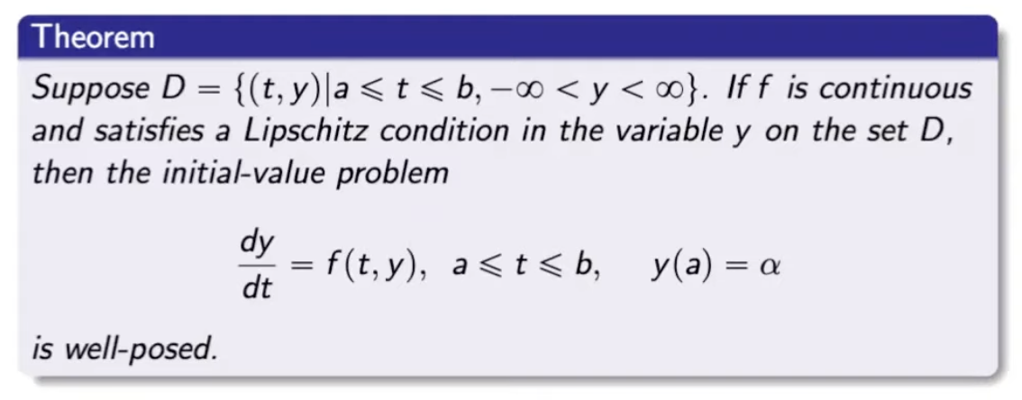
  A function \(f(t, y)\) is said to satisfy a Lipschitz condition in the variable \(y\) on a set \(D \subset \mathbb R^2\) if a constant \(L > 0\) exists with \(\mid f(t, y_1) - f(t, y_2) \mid \leq L\mid y_1 - y_2 \mid\)

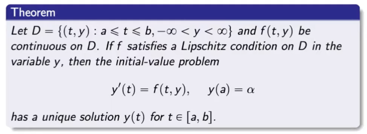
  IVP is well-posed if it has a unique solutions, and an IVP obtained by small perturbations also has a unique solution. We consider IVPs of the form \(dy/dt = f(t, y)\), \(a \leq t \leq b\), \(y(a) = \alpha\).

  

• Euler’s method - We generate mesh points and interpolate. As we are considering IVPs of a certain form, we can just use 1st degree Taylor’s polynomial to approximate the solution to the IVP. We take \(q_0 = \alpha\) and \(w_{i + 1} = w_i + hf(t_i, w_i)\) for \(i \geq 0\) where \(w_i \approx y(t_i)\). The error grows as \(t\) increases, but it is controlled due to the stability of Euler’s method. It grows in a linear manner wrt to \(h\).

• Error in Euler’s method - Suppose \(\mid y''(t) \mid \leq M\), then \(\mid y(t_i) - w_i \mid \leq \frac{hM}{2L}(\exp (L(t_i - a)) - 1)\). What about round-off errors? We’ll get an additional factor of \(\delta/hL\) in the above expression along with the constant \(\delta_0 \exp (L(t_i - a))\). Therefore, \(h = \sqrt(2\delta/M)\).

• Local truncation error - \(\tau_{i + 1}(h) = \frac{y_{i + 1} - y_i}{h} - \phi(t_i, y_i)\). It is just \(hM/2\) for Euler’s method (\(\phi\) refers to the Taylor polynomial). We want truncation error to be as \(\mathcal O(h^p)\) for as large \(p\) as possible.

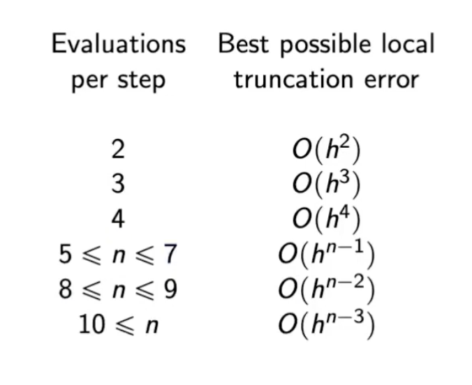
  Higher order Taylor methods - Assume \(f\) is \(n\)-times continuously differentiable. We get \(\mathcal O(n)\) for \(n\)th degree Taylor polynomial. However, the number of computations are a bit high.

  Practice problems on this

• What about interpolation? We should use cubic Hermite interpolation (to match the derivative too).

• Now, we try to reduce the computation of higher order derivatives. Runge-Kutta methods - Based off Taylor’s theorem in two variables.

  

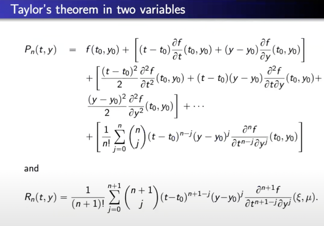
  Order 2- We get \(a = 1, \alpha = h/2, \beta = f(t, y)h/2\) by equating \(af(t + \alpha, y + \beta)\) to \(T(t, y) = f(t, y) + h/2 f'(t, y)\). This specific Runge-Kutta method of Order 2 is known as the midpoint-method. (2D of Taylor order 2) \(w_{i + 1} = w_i + hf\left(t_i + \frac{h}{2}, w_i + \frac h 2 f(t_i, w_i)\right)\) The number of nesting \(f\)‘s represents the order of the differential equation.

  Suppose we try the form \(a_1f(t, y) + a_2 f(t + \alpha_2, y + \delta_2 f(t, y))\) containing 4 parameters to approximate. We still get \(\mathcal O(n^2)\) as there is only one nesting.

• However, the flexibility in the parameters allows us to derive the Modified Euler method. \(w_{i + 1} = w_i + \frac h 2[f(t_i, w_i) + f(t_{i + 1}, w_i + hf(t_i, w_i))]\) Higher-order Runge-Kutta methods - The parameter values are used in the Heun’s method.

  

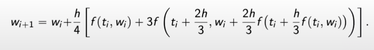
  The most common Runge-Kutta is order 4 whose local truncation error is \(\mathcal O(n^4)\).

  

• Error control in Runge-Kutta methods. Adaptive step size for lower error. Single step approximation - uses \(i-\) for \(i\). Given an \(\epsilon > 0\), we need to be able to give a method that gives \(\mid y(t_i) - w_i\mid < \epsilon\). \(y(t_{i + 1}) = y(t_i) + h\phi(t_i, y(t_i), h) + \mathcal O(h^{n + 1}) \\\) Local truncation error assumes \(i\)th measurement is correct to find error in the \(i + 1\)th measurement. We get \(\tau_{i + 1}(h) \approx \frac 1 h (y(t_{i + 1}) - w_{i + 1})\) assuming \(y_i \approx w_i\). For \(n\)th degree truncation error, we get \(\tau_{i + 1}(h) \approx \frac 1 h (w^{n + 1}_{i + 1} - w^{n}_{i + 1})\). After a few approximations, we get that the local truncation error changes by a factor of \(q^n\) when the step size changes by a factor of \(q\).

• Runge-Kutta-Fehlberg Method - It uses a Runge-Kutta method with local truncation error of order five. We change the step size if \(q < 1\). These methods are just an analogue of adaptive quadrature methods of integrals.

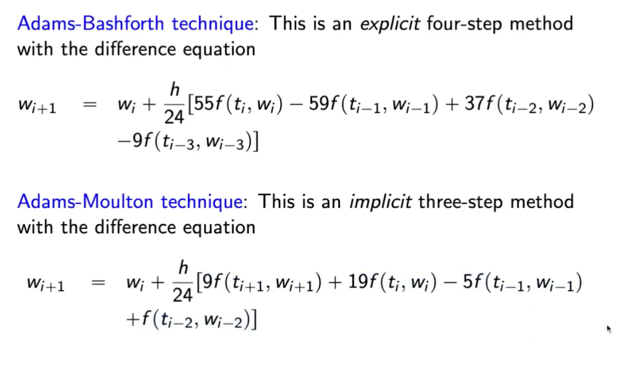
• Multi-step methods. Methods that use the approximation at more than one previous mesh point to determine the approximation at the next point. The general equation is implicit where \(w_{i + 1}\) occurs on both sides of the equation. Implicit methods are more accurate than explicit methods.

  

• Predictor-Corrector Method - How do we solve implicit methods? We can use the root-finding procedures we learnt. All of this can get quite cumbersome. We just use implicit methods to improve the prediction of the explicit methods. We insert the solution of explicit method (prediction) and insert it on the rhs of the implicit method (correction).

• Consistency and Convergence

  One-step difference method is consistent if \(\lim_{h \to 0}\max_{1 \leq i \leq n}\mid \tau_i(h)\mid = 0\). But we also need the global measure - convergence - \(\lim_{h \to 0}\max_{1 \leq i \leq n}\mid y_i(t_i) - w_i\mid = 0\)

  stability considering round-off errors. For the function \(\phi\) satisfying Lipschitz condition with a \(h_0\), the one-step difference method is convergent iff it is consistent. The local truncation error is bounded, and we get \(\mid y(t_i) - q_i \mid \leq \frac {\tau(h)}{L}e^{L(t_i - a)}\).

  Analysis of consistency, convergence, and stability is difficult for multi-step methods. Adams-* methods are stable.

• Numerical Linear Algebra - Basics - \(Ax = b\) has a unique solution iff \(A\) is invertible, and it does not have a unique or has no solution otherwise.

  Cramer’s rule - \(x_j = \frac{\det A_j}{\det A}\). However, this is cumbersome. Determinant of an upper triangular matrix is product of the diagonal entries.

  Gaussian Elimination Method - \(A = LU\) for most matrices \(A\). \(L\) is a lower triangular matrix and \(U\) is an upper triangular matrix. Form the augmented matrix \([ A \mid b]\). Linear combination of rows and swapping of rows can be performed. What is the total number of arithmetic operations?

  For converting to triangular - We use \((n - i)\) divisions for each row and \((n - i + 1)\) multiplications for each column of each row. Also, we have \((n - i)(n - i + 1)\) subtractions. In total, we have \((n - i)(n - i + 2)\) multiplications. Summing, we get \(\mathcal O(n^3)\) multiplications (\((2n^3 + 3n^2 - 5n)/6\)) and subtractions \(((n^3 - n)/3)\).

  For back substitution - multiplication is \((n^2 + n)/2\) and subtraction is \((n^2 - n)/2\).

• We have not considered finite digit arithmetic for GEM previously. The error dominates the solution when the pivot has a low absolute value. In general, we need to ensure that the pivot does not have very low magnitude by interchanging rows (followed by interchanging columns for triangular form if needed) - partial pivoting. However, this might not be enough to get rid of the rounding error. Therefore, we need to consider scaled partial pivoting. Define \(s_i\) as the maximum magnitude in the \(i\)th row. Now, the first pivot is chosen by taking the row with the maximum value of \(a_{i1}/s_i\). The operation count order still remains the same. You need not calculate scale factors more than once.

• LU Decomposition - The conversion of \(A\) to a triangular form using the above method can be represented as a sequence of matrix multiplications (if \(A\) does not require any row interchanges). The inverse of a matrix depicting operations on \(A\) can be seen a matrix depicting the same inverse operations on \(A\). In the end, we get \(A = (L^{(1)} \dots L^{(n - 1)})(M^{(1)}\dots M^{(n-1)}A)\) where each \(M^{(i)}\) represents the action that uses \(A_{ii}\) as a pivot. Once we get \(L\) and \(U\), we can solve \(y = Ux\) and \(Ly = b\) separately. There are multiple decompositions possible which are eliminated by imposing conditions on the triangular matrices. One such condition is setting \(L_{ii} = U_{ii}\) which is known as Cholesky Decomposition.

  We had assumed that row interchanges are not allowed. However, we can build permutation matrices for row interchanges which will be of the form of an identity matrix with row permutations.

  Therefore, we get PLU decomposition.

• Diagonally dominant matrices - An \(n \times n\) matrix \(A\) is said to be diagonally dominant when \(\mid a_{ii} \mid \geq \sum^n \mid a_{ij} \mid\) for all rows. A strongly diagonally dominant matrix is invertible. Such matrices will not need row interchanges, and the computations will be stable wrt the round off errors.

  Why this instead of \(\mid a_{ii} \mid \geq \max \mid a_{ij} \mid\)

  A matrix \(A\) is positive definite if \(x^tAx > 0\) for every \(x \neq 0\). We shall also consider \(A\) to be symmetric in the definition. Every positive definite matrix is invertible, \(A_{ii} > 0\) for each \(i\), \((A_{ij})^2 < A_{ii}A_{jj}\), and \(\max_{1\leq k, j \leq n} \mid A_{kj} \mid \leq \max_{1 \leq i \leq n}\mid A_{ii}\mid\).

  A leading principal submatrix of matrix \(A\) is the top-left \(k \times k\) submatrix of \(A\). \(A\) is positive definite iff each leading principal submatrix of \(A\) has a positive determinant.

  Gaussian Elimination on a symmetric matrix can be applied without interchanging columns iff the matrix is positive definite.

  A matrix \(A\) is positive definite iff \(A = LDL^t\) where \(L\) is lower triangular with 1’s on the diagonal and \(D\) is a diagonal matrix with positive diagonal entries. Alternatively, \(A\) is positive dfinite iff \(A = LL^t\) where \(L\) is a lower triangular matrix. Note. Positive definite is stronger than Cholesky decomposition.

• We have been seeing direct methods for solving \(Ax = b\). We shall see some iterative methods now. We need a distance metric to check the closeness of the approximation. We will consider \(l_2\) distance = \(\| x - y\|_2 = \left( \sum_{i = 1}^n (x_i - y_i)^2 \right)^{1/2}\) and \(l_\infty\) distance = \(\| x - y\|_2 = \max_{i = 1}^n \mid x_i - y_i \mid\). Also, \(\|x - y\|_\infty \leq \|x - y\|_2 \leq \sqrt n\|x - y\|_\infty\). We also need to consider distances in matrices.

• Distances in Matrices - \(\|A\|_2 = \max_{\|x\|_2 = 1} \|Ax\|_2\) and \(\|A\|_\infty = \max_{\|x\|_\infty = 1} \|Ax\|_\infty\). The \(l_\infty\) can be directly calculated using \(\|A\|_\infty = ]max_{i} \sum_j \mid A_{ij} \mid\).

• eigenvalues, eigenvectors - A non-zero vector \(v \in \mathbb R^n\) is an eigenvector for \(A\) if there is a \(\lambda \in \mathbb R\) such that \(Av = \lambda v\) and \(\lambda \in \mathbb R\) is the eigenvalue. The characteristic polynomial of \(A\) is \(\det(A - \lambda I)\). We do not consider the complex roots that are not real for these polynomials to calculate eigenvalues.

  Spectral radius - \(\rho(A) = \max \mid \lambda \mid\). Then, we have the relation that \(\|A\|_2 = [\rho(A^tA)]^{1/2}\) and also \(\rho(A) \leq \|A\|_2\) and \(\rho(A) \leq \|A\|_\infty\).

  Convergent matrices - It is of particular importance to know when powers of a matrix become small, that is, when all the entries approach zero. An \(n \times n\) matrix \(A\) is called convergent if for each \(1 \leq i, j \leq n\), \(\lim_{k \to \infty}(A^k)_{ij} = 0\).

  • \(A\) is a convergent matrix
  • \[\lim_{n \to \infty} \|A^n\|_2 = 0\]
  • \[\lim_{n \to \infty} \|A^n\|_\infty = 0\]
  • \[\rho(A) < 1\]
  • \(\lim_{n \to \infty} A^nv =0\) for every vector \(v\).

  The above statements are all equivalent.

• Iterative techniques are not often used for smaller dimensions. We will study Jacobi and the Gauss-Seidel method.

  Jacobi Method - We assume that \(\det(A)\) being non-zero (as matrix must be invertible for solution) and the diagonal entries of \(A\) are also non-zero. We have

  Jacobi suggested that we start with an initial vector \(x^{(0)} = [x_1^{(0)}, \dots, x_n^{(0)}]\) and for \(k \geq 1\)

  \[x_i^{(k)} = \frac{b_i - \sum_{j \neq i} a_{ij}x_j^{(k - 1)}}{a_{ii}}\]

  The error in the iterations is given by

  \[\mid x_i - x_i^{(k)} \mid \leq (\sum_{j \neq i} \frac{a_{ij}}{a_{ii}})\|x_j - x_j^{(k - 1)}\|_\infty\]

  which gives

  \[\| x - x^{(k)} \|_\infty \leq (\max_i \sum_{j \neq i} \frac{a_{ij}}{a_{ii}})\|x_j - x_j^{(k - 1)}\|_\infty\]

  If \(\mu = \max{i}\sum_{j \neq i} \frac{a_{ij}}{a_{ii}} < 1\), then convergence is guaranteed. If \(\mu < 1\), then the condition is nothing but that of strictly diagonally dominant matrices.

  Gauss-Seidel method - The idea is that once we have improved one component, we use it to improve the component of the next component and so on.

  \[x_i^{(k)} = \frac{1}{a_{ii}} \left[b_i - \sum_{j = 1}^{i - 1}a_{ij}x_j^{(k)} - \sum_{j = i + 1}^n a_{ij}x_j^{(k - 1)}\right]\]

  There are linear systems where Jacobi method converges but Gauss-Seidel method does not converge. If \(A\) is strictly diagonally dominant, then both methods converge to the true solution.

• Residual vector - If \(\tilde x\) is an approximation to \(Ax = b\), then \(r = b - A\tilde x\) is the residual vector. However, it is not always true that when \(\|r \|\) is small then \(\|x - \tilde x\|\) is also small. This is because \(r = A(x - \tilde x)\), and that represents the affine transformation of space. This phenomenon is captured as follows

  For a non-singular \(A\), we have

  \[\|x - \tilde x\|_\infty \leq \|r \|_\infty \cdot \|A^{-1}\|_\infty\]

  If \(x \neq 0\) and \(b \neq 0\)

  \[\frac{\|x - \tilde x \|_\infty}{\|x\|_\infty} \leq \|A\|_\infty\cdot \|A^{-1}\|_\infty \cdot \frac{\|r\|_\infty}{\|b\|_\infty}\]

  These relations work for \(l_2\) norm too.

  I think \(\|A\|_\infty \|x\|_\infty \geq \|b\|_\infty\)

  The condition number of a non-singular matrix \(A\) is

  \[K(A) = \|A\|_\infty \cdot \|A^{-1}\|_\infty\]

  Also, \(\|AA^{-1}\|_\infty \leq \|A\|_\infty \|A^{-1}\|_\infty\). A non-singular matrix \(A\) is said to be well-conditioned if \(K(A)\) is close to 1.

  However, the condition number depends on the round-off errors too. The effects of finite-digit arithmetic show up in the calculation of the inverse. As the calculation of inverse is tedious, we try to calculate the condition number without the inverse. If we consider \(t\)-digit arithmetic, we approximately have

  \[\|r\|_\infty \approx 10^{-t}\|A\|_\infty \cdot \|\tilde x \|_\infty\]

  One drawback is that we would have to calculate \(r\) is double precision due to the above relation. The approximation for \(K(A)\) comes from \(Ay = r\). Now, \(\tilde y \approx A^{-1}r = x - \tilde x\). Then,

  \[\|\tilde y\| \leq \|A^{-1}\| \cdot (10^{-t}\cdot \|A\| \|\tilde x\|)\]

  Using the above expression, we get

  \[K(A) \approx \frac{\|\tilde y\|}{\|\tilde x\|}10^t\]

  The only catch in the above method is that we need to calculate \(r\) in \(2t\)-finite arithmetic.

  Iterative refinement - As we had defined \(\tilde y = x - \tilde x\), in general, \(\tilde x + \tilde y\) is more accurate. This is called as iterative improvement. If the process is applied using \(t\)-digit arithmetic and if \(K(A) \approx 10^q\), then after \(k\) iterations, we have approximately \(\min(t, k(t - q))\) correct digits. When \(q> t\), increased precision must be used.

• Approximations for eigenvalues

  Gerschgorin theorem - We define discs \(D_i = \left\{ z \in \mathbb C: \mid z - a_{ii} \mid \leq \sum_{j \neq i} \mid A_{ij} \mid \right\}\). Then, all eigenvalues of \(A\) are contained in the union of all the disks \(D_i\). The union of any \(k\) of the disk that do not intersect the remaining \(n - k\) disks contains precisely \(k\) of the eigenvalues including the multiplicity. From this theorem, we get that strictly diagonally dominant matrices are invertible. This is also true for strictly diagonally column dominant matrices.

  The above theorem provides us the initial approximations for the eigenvalues. We shall see the Power method.

  Power method - We assume \(\mid \lambda_1 \mid > \mid \lambda_2 \mid \geq \dots \geq \mid \lambda_n \mid\), and that \(A\) has \(n\) linearly independent eigenvectors. Choose a non-zero \(z \in V\), and compute

  \[\lim_{k \to \infty} A^k z\]

  to get the eigenvalue! (Think of vector space transformations geometrically).

  If \(z = \sum \alpha_i v_i\), we get

  \[A^k z = \lambda^k_1 \alpha_1 v_1 + \dots + \lambda^k_n \alpha_n v_n = \lambda_1^k \alpha_1 v_1\]

  for high values of \(k\).

  Sometimes, \(z\) may not have the component of \(v_1\). We choose a vector such that this is not the case.

  Sometimes, it may also be the case that

  \(\mid \lambda_1 \mid \geq \mid \lambda_2 \mid \geq \dots > \mid \lambda_n \mid > 0\). \(A\) is invertible iff this holds. Then, we use the power method on \(A^{-1}\).

  Sometimes, \(\mid \lambda_1 \mid < 1\) and we’ll converge to 0. On the other hand, if it is more than 1, the limit will shoot to infinity. To take care of these, we scale \(A^k(z)\), so that it is finite and non-zero.

  Firstly, we choose \(z\) such that \(\|z^{(0)}\| = 1\) and we choose a component \(p_0\) of \(z^{(0)}\) such that \(\mid z_{p_0}^{(0)} \mid = 1\). Following this, we scale each subsequent value as follows - Let \(w^{(1)} = Az^{(0)}\) and \(\mu^{(1)} = w_{p_0}^{(1)}\).

  \[\mu^{(1)} = \lambda_1 \frac{\alpha_1(v_1)_{p_0} + \dots + (\lambda_n/ \lambda_1) \alpha_n (v_n)_{p_0}}{\alpha_1(v_1)_{p_0} + \dots + \alpha_n (v_n)_{p_0}}\]

  Now, we choose \(p_1\) to be the least integer with \(\mid w_{p_1}^{(1)}\mid = \|w^{(1)}\|\) and define \(z^{(1)}\) by

  \[z^{(1)} = \frac{1}{w_{p_1}^{(1)}} Az^{(0)}\]

  Then, in general,

  \[\mu^{(m)} = w_{p_{m - 1}}^{(m)} = \lambda_1 \frac{\alpha_1(v_1)_{p_0} + \dots + (\lambda_n/ \lambda_1)^m \alpha_n (v_n)_{p_0}}{\alpha_1(v_1)_{p_0} + \dots + (\lambda_n/ \lambda_1)^{m - 1}\alpha_n (v_n)_{p_0}}\]

  Now, \(\lim_{m \to \infty} \mu^{(m)} = \lambda_1\).

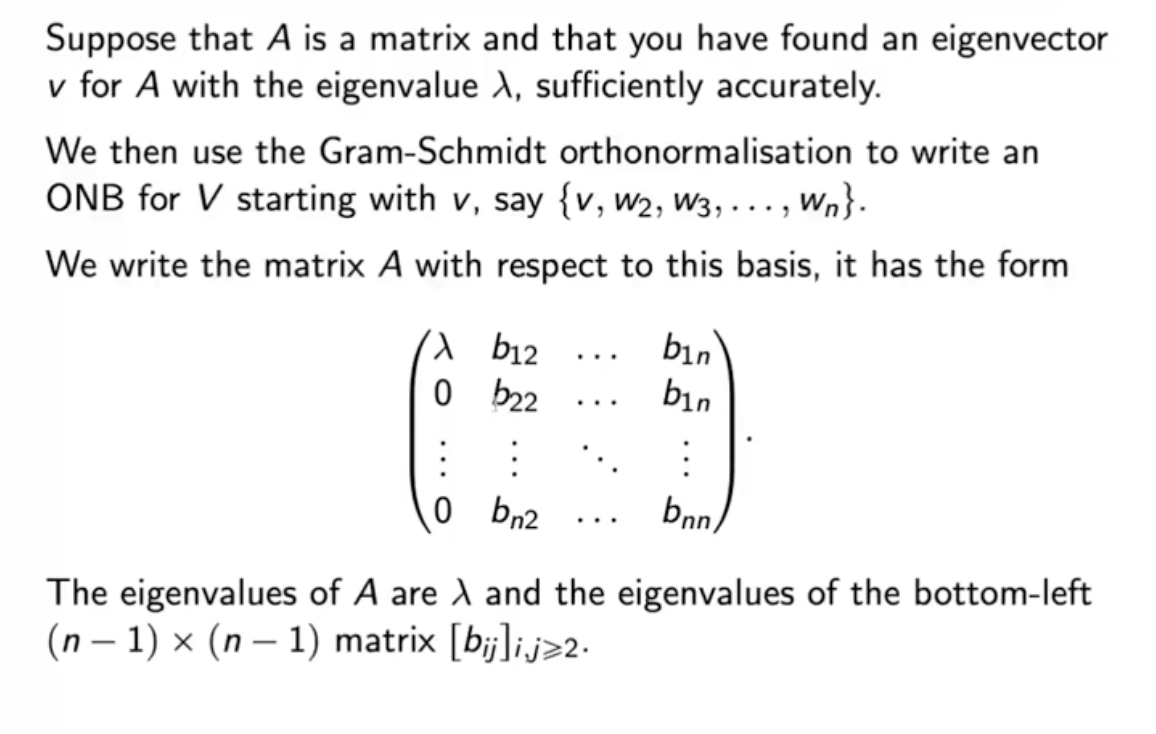
  To find other eigenvalues, we use Gram-Schmidt orthonormalisation.

  

---

END OF COURSE

---