Object Detection
What objects are where? Object detection can be performed using either traditional (1) image processing techniques or modern (2) deep learning networks.
- Image processing techniques generally don’t require historical data for training and are unsupervised in nature. OpenCV is a popular tool for image processing tasks.
- Pros: Hence, those tasks do not require annotated images, where humans labeled data manually (for supervised training).
- Cons: These techniques are restricted to multiple factors, such as complex scenarios (without unicolor background), occlusion (partially hidden objects), illumination and shadows, and clutter effect.
- Deep Learning methods generally depend on supervised or unsupervised learning, with supervised methods being the standard in computer vision tasks. The performance is limited by the computation power of GPUs, which is rapidly increasing year by year.
- Pros: Deep learning object detection is significantly more robust to occlusion, complex scenes, and challenging illumination.
- Cons: A huge amount of training data is required; the process of image annotation is labor-intensive and expensive. For example, labeling 500’000 images to train a custom DL object detection algorithm is considered a small dataset. However, many benchmark datasets (MS COCO, Caltech, KITTI, PASCAL VOC, V5) provide the availability of labeled data.
The field of object detection is not as new as it may seem. In fact, object detection has evolved over the past 20 years. The progress of object detection is usually separated into two separate historical periods (before and after the introduction of Deep Learning):
- Object Detector Before 2014 – Traditional Object Detection period
- Viola-Jones Detector (2001), the pioneering work that started the development of traditional object detection methods
- HOG Detector (2006), a popular feature descriptor for object detection in computer vision and image processing
- DPM (2008) with the first introduction of bounding box regression Object Detector
- After 2014 – Deep Learning Detection period Most important two-stage object detection algorithms
- RCNN and SPPNet (2014) - Region CNN
- Fast RCNN and Faster RCNN (2015)
- Mask R-CNN (2017)
- Pyramid Networks/FPN (2017)
- G-RCNN (2021) - Granulated RCNN
- Most important one-stage object detection algorithms
- YOLO (2016)
- SSD (2016)
- RetinaNet (2017)
- YOLOv3 (2018)
- YOLOv4 (2020)
- YOLOR (2021)
- YOLOv7 (2022)
- YOLOv8 (2023)
In general, deep learning based object detectors extract features from the input image or video frame. An object detector solves two subsequent tasks:
- Task #1: Find an arbitrary number of objects (possibly even zero), and
- Task #2: Classify every single object and estimate its size with a bounding box.
YOLO - You Only Look Once
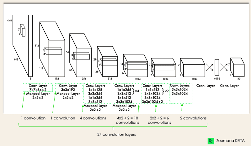
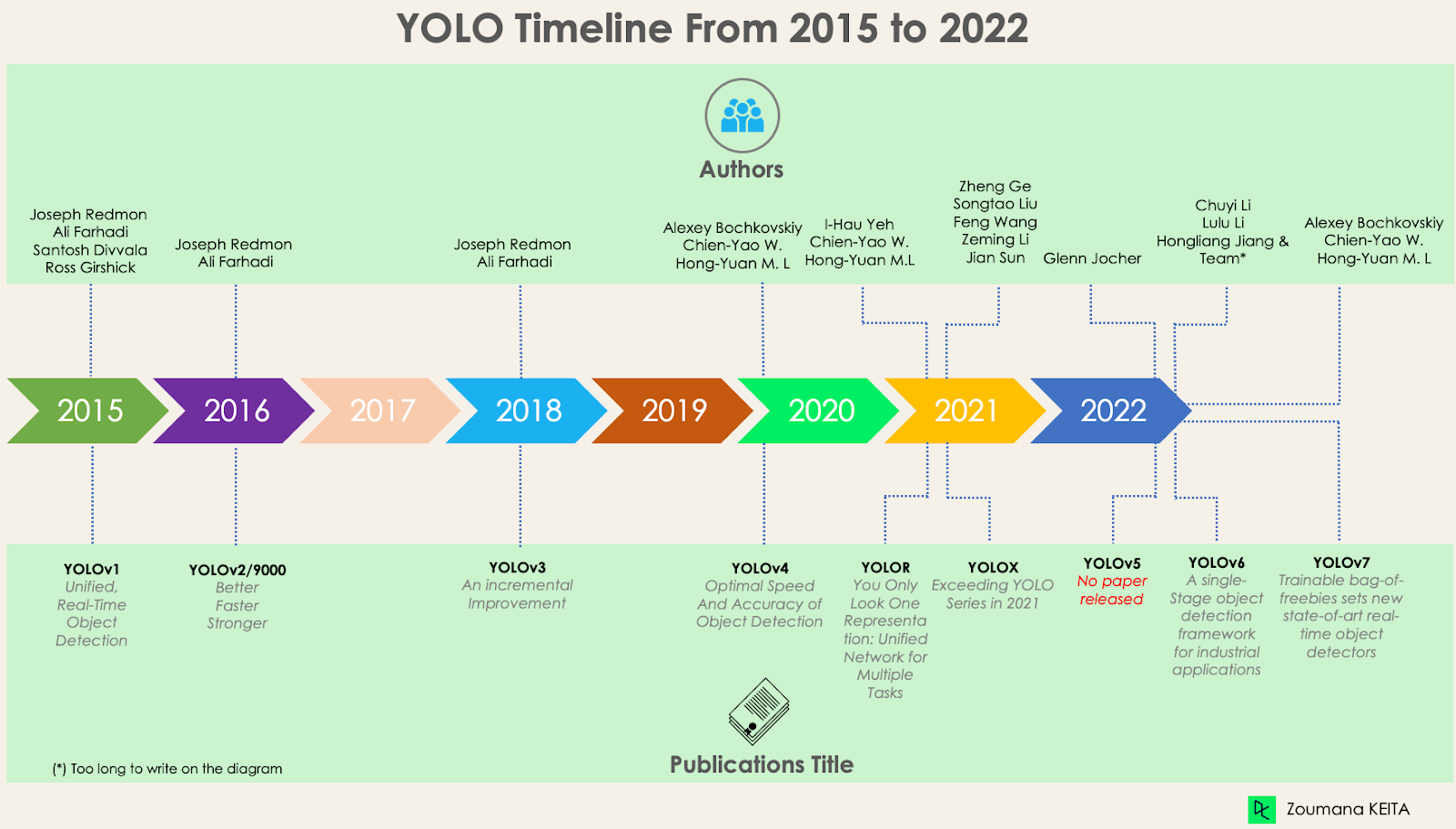
It is a popular family of real-time object detection algorithms. The original YOLO object detector was first released in 2016. It was created by Joseph Redmon, Ali Farhadi, and Santosh Divvala. At release, this architecture was much faster than other object detectors and became state-of-the-art for real-time computer vision applications.
The algorithm works based on the following four approaches:
-
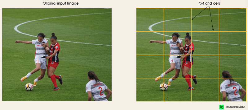
Residual blocks - This first step starts by dividing the original image (A) into NxN grid cells of equal shape, where N in our case is 4 shown on the image on the right. Each cell in the grid is responsible for localizing and predicting the class of the object that it covers, along with the probability/confidence value.
-
Bounding box regression -
The next step is to determine the bounding boxes which correspond to rectangles highlighting all the objects in the image. We can have as many bounding boxes as there are objects within a given image.
YOLO determines the attributes of these bounding boxes using a single regression module in the following format, where Y is the final vector representation for each bounding box.
\[Y = [pc, bx, by, bh, bw, c1, c2]\]where \(pc\) is the probability score of the grid containing the object. \(c1, c2\) correspond to the object classes - ball and player.
-
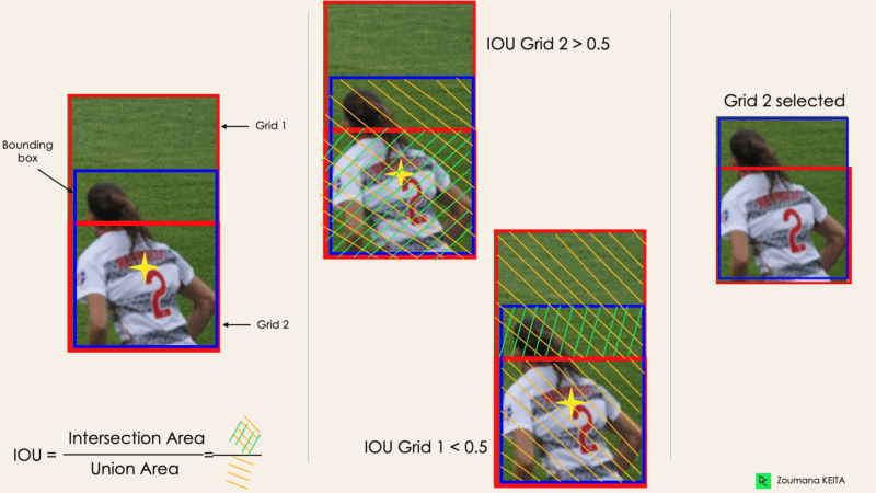
Intersection Over Unions or IOU for short
Most of the time, a single object in an image can have multiple grid box candidates for prediction, even though not all of them are relevant. The goal of the IOU (a value between 0 and 1) is to discard such grid boxes to only keep those that are relevant. Here is the logic behind it:
- The user defines its IOU selection threshold, which can be, for instance, 0.5.
- Then YOLO computes the IOU of each grid cell which is the Intersection area divided by the Union Area.
- Finally, it ignores the prediction of the grid cells having an IOU ≤ threshold and considers those with an IOU > threshold.
-
Non-Maximum Suppression.
Setting a threshold for the IOU is not always enough because an object can have multiple boxes with IOU beyond the threshold, and leaving all those boxes might include noise. Here is where we can use NMS to keep only the boxes with the highest probability score of detection.
Although YOLO was state-of-the-art when it released, with much faster detection, it had a few disadvantages. It is unable to detect smaller objects within a grid as each grid is designed for single object detection. It is unable to detect new or unusual shapes, and the same loss function is used for both small and large bounding boxes which creates incorrect localizations.
YOLOv2 improvised over the existing architecture using Darknet-19 as new architecture (Darknet is an open-source neural network framework in C and CUDA),
- batch normalization - reduced overfitting using a regularization effect.
- higher resolution of inputs,
- convolution layers with anchors - Replaces fully connected laters with anchor boxes to prevented predicting the exact coordinate of bounding boxes. Recall improved, accuracy decreased. Anchor boxes are predefined grids with certain aspect ratios spatially located in an image. These boxes are checked for an object probability score and are selected accordingly.
- dimensionality clustering - The previously mentioned anchor boxes are automatically found by YOLOv2 using k-means dimensionality clustering with k=5 instead of performing a manual selection. This novel approach provided a good tradeoff between the recall and the precision of the model.
- Fine-grained features - YOLOv2 predictions generate 13x13 feature maps, which is of course enough for large object detection. But for much finer objects detection, the architecture can be modified by turning the 26 × 26 × 512 feature map into a 13 × 13 × 2048 feature map, concatenated with the original features.
YOLOv3 is an incremental improvement using Darknet-53 instead of Darknet-19. YOLOv4 is an optimized for parallel computations. This architecture, compared to YOLOv3, adds the following information for better object detection:
- Spatial Pyramid Pooling (SPP) block significantly increases the receptive field, segregates the most relevant context features, and does not affect the network speed.
- Instead of the Feature Pyramid Network (FPN) used in YOLOv3, YOLOv4 uses PANet for parameter aggregation from different detection levels.
- Data augmentation uses the mosaic technique that combines four training images in addition to a self-adversarial training approach.
- Perform optimal hyper-parameter selection using genetic algorithms.
YOLOR is based on the unified network which is a combination of explicit and implicit knowledge approaches - (1) feature alignment, (2) prediction alignment for object detection, and (3) canonical representation for multi-task learning.
Then, YOLOX, using a modified version of YOLOv3, decoupled classification and localization increasing the performance of the model. Mosaic and MixUp data augmentation approaches were added. Removed the anchor-based system that used to perform clustering under the hood. Introduced SimOTA instead of IoU.
YOLOv5 uses Pytorch rather than Darknet, and has 5 different model sizes. YOLOv6 was developed for industrial applications and introduced three improvements - a hardware-friendly backbone and neck design, an efficient decoupled head, and a more effective training strategy.
YOLOv7 - Trained bag-of-freebies sets new state-of-the-art for real-time object detectors. It reformed the architecture by integrating Extended Efficient Layer Aggregation Network (E-ELAN) which allows the model to learn more diverse features for better learning. The term bag-of-freebies refers to improving the model’s accuracy without increasing the training cost, and this is the reason why YOLOv7 increased not only the inference speed but also the detection accuracy.
R-CNN - Region-based Convolutional Neural Networks
R-CNN models first select several proposed regions from an image (for example, anchor boxes are one type of selection method) and then label their categories and bounding boxes (e.g., offsets). These labels are created based on predefined classes given to the program. They then use a convolutional neural network (CNN) to perform forward computation to extract features from each proposed area.
In 2015, Fast R-CNN was developed to significantly cut down train time. While the original R-CNN independently computed the neural network features on each of as many as two thousand regions of interest, Fast R-CNN runs the neural network once on the whole image. This is very comparable to YOLO’s architecture, but YOLO remains a faster alternative to Fast R-CNN because of the simplicity of the code.
At the end of the network is a novel method known as Region of Interest (ROI) Pooling, which slices out each Region of Interest from the network’s output tensor, reshapes, and classifies it (Image Classification). This makes Fast R-CNN more accurate than the original R-CNN.
Mask R-CNN is an advancement of Fast R-CNN. The difference between the two is that Mask R-CNN added a branch for predicting an object mask in parallel with the existing branch for bounding box recognition. Mask R-CNN is simple to train and adds only a small overhead to Faster R-CNN; it can run at 5 fps.
Other Approaches
SqueezeDet was specifically developed for autonomous driving, where it performs object detection using computer vision techniques. Like YOLO, it is a single-shot detector algorithm. In SqueezeDet, convolutional layers are used only to extract feature maps but also as the output layer to compute bounding boxes and class probabilities. The detection pipeline of SqueezeDet models only contains single forward passes of neural networks, allowing them to be extremely fast.
MobileNet is a single-shot multi-box detection network used to run object detection tasks. This model is implemented using the Caffe framework.
References
Enjoy Reading This Article?
Here are some more articles you might like to read next: