Introduction

The content on this article is based on the course by Prof. Prithviraj at UC San Diego. This whitepaper about AI Agents by Google is also a good read.

What is an agent?

Agent is an entity with agency. A Minecraft agent?. Agents see applications within the workspaces in the form of workflow automations, household or commercial robotics, software development and personal assistants. Generally, the theme is that agents take actions.

Historically, the use of agents started in the early 1900s in the field of control theory. They were used for dynamic control of flight systems, and in 1940s it expanded to flight guidance, etc. By the 1950s the concepts of MDPs and dynamic programming were being expanded to many use cases. Surprisingly, one of the first natural language chatbots, Eliza, was created as a psychotherapist simulator in the 1960s! Finally, reinforcement learning became a field of study in the 1990s for sequential decision making.

Sequential Decision Making

These tasks are different from other ML problems like classification. A model that has an accuracy of 99% at each step, has a cumulative accuracy of ~30% after 120 steps!

These problems are formalized as a Markov Decision Process - an agent performs actions in an environment, and in turn receives rewards as feedback. These configurations are distinguished as states, and the whole process can be seen as sequential decision making.

The core components of an agent, often agreed on, are

Grounding - Language is anchored to concepts in the world. Language can be grounded to different forms of information systems - images, actions and cultural norms.
- Agency (ability to act) - At each state, an agent needs to have multiple choices to act. If an agent has to select what tools to use but there’s always only one tool, is that agency? The action space has to be well-defined to look for agency. Although there is a single tool call, different parameters for the tool call can probably be considered as different actions. Actions can be defined as something the agent does and changes the environment. The distinction between an agent and environment is not very clear in many cases. Although, our approximations mostly serve us well.
- Planning (Long horizon)
- Memory -
  - Short-term - What is the relevant information around the agent that it needs to use to act now
  - Long term - What information has the agent already gathered that it can retrieve to take an action
- Learning (from feedback) - Doesn’t necessarily always mean backpropagation.
Additional -
- Embodiment (physically acting in the real-world). Embodied hypothesis - embodiment is necessary for AGI.
- Communication - Can the agent communicate its intentions to other agents. Very necessary pre-requisite for multi-agent scenarios.
- World Modeling - Given the state of the world and an actions, predict the next state of the world. Is Veo/Sora a world model? It is an attempt for world model since they have no verifiability. Genie is another such attempt. So is Genesis - this is much better if it works.
- Multi-modality - The clean text on the internet is only a few terabytes, and our models have consumed it (took use 2 decades though). YouTube has 4.3 Petabytes of new videos a day. CERN generates 1 Petabyte a day (modalities outside vision and language). Some people believe this form of scaling is the way to go. There are more distinctions -

Model	AI System	Agent
GPT-4	ChatGPT	ChatGPT computer use
Forward passes of a neural net	Mixing models together	Has agency

It is important to remember that not every use case needs an agent and most use cases just need models or AI systems. Occam’s razor.

Simulated Environments and Reality

Why do we need simulations? Most tasks have many ways of completing them. There is no notion of global optimal solutions ahead of time but usually known once the task is complete.

The agent needs to explore to find many solutions to compare and see what is the most efficient. However, exploration in the read world is expensive - wear and tear of robots, excessive compute, danger to humans, etc.

Simulations offer an easy solution to these problems. Assign a set of rules, and let a world emerge. One of the early examples of this is Conway’s Game of Life which theorized that complicated behaviors can emerge by just a few rules.

From an MDP perspective, a simulation contains $<S, A, T>$ where

$S$ is the set of all states. It consists of propositions that are true/false. Example: You are in a house, door is open, knife in drawer
$A$ is the set of all actions. Example: Take knife from drawer, walk through door
$T$ is the transition matrix - (You are in the house, you walk out of the door) -> You are outside the house.

A simulation need not have an explicit reward.

Sim2Real Transfer

The ability of an agent trained in simulation transfer to reality is dependent on how good the model extrapolates out of distribution. With the current stage of agents, the simulation is made as close to reality as possible to reduce the Sim2Real gap.

How do we measure closeness to reality? The tasks in the real world have different types of complexities -

Cognitive complexity - Problems that requires long chains of reasoning - puzzles, math problems or moral dilemmas
Perceptive complexity - Requires high levels of vision and/or precise motor skills - bird watching, threading a needle, Where’s Waldo

Examples of simulations -

Grid world - low cognitive and almost zero perceptive. However, this idea can arbitrarily scale to test algorithms for their generalization potential in controllable settings.
Atari - low perceptive, medium cognitive. Atari games became very popular in 2013, when Deepmind released their Deep Q-Net paper that achieved human level skills on these games.
Zork, NetHack - low perceptive, high cognitive. These are configurations or worlds that you purely interact with text. The worlds are actually so complex that there is no agent that is able to finish the challenge!
Clevr simulation - medium perceptive, low cognitive - This simulation generates images procedurally with certain set of objects and has reasoning questions for each image.
AI2 THOR - medium perceptive, medium cognitive. Worlds with ego-centric views for robotics manipulation and navigation simulations
AppWorld - medium perceptive, medium cognitive. A bunch of different apps that you would generally use in daily life. The agents can access apps, and the simulation also has human simulators. This simulation is one that is closest to reality in the discussed so far!
Minecraft - medium perceptive, high cognitive. A voxel based open-world game that lets players take actions similar to early-age humans.
Mujoco - high perceptive, low cognitive. It is a free and open source physics engine to aid the development of robotics.
Habitat - high perceptive, medium cognitive. A platform for research in embodied AI that contains indoor-world ego-centric views similar to AI2 THOR, but with much better graphics. They have recently added sound in the environment too!
High perceptive, high cognitive - Real world, and whoever gets this simulation right, wins the race to AGI. It requires people to sit down and enumerate all kinds of rules. Game Engines like Unreal and Unity are incredibly complex, and are the closest we’ve gotten.

Some researchers try to “learn” the simulations from real-world demonstrations.

In each of these simulators, think of the complexity and reward sparsity in the environment. It is easy to build a simulator that gives rewards at a goal state than the one that gives a reward for each action. There are some open-lines of research in this domain -

Which dimensions of complexity transfer more easily? Curriculum learning
Can you train on lower complexity and switch to a higher complexity?
Can we learn the world model holy grail?

How to make simulations?

As we’ve seen, simulations can range from games to real-world replications with physics involved. Most simulations are not designed keeping AI in mind. However, with the current state of AI, this is an important factor to keep in mind.

Classical environments like in Zork/AI2 Thor/Mujoco have something known as PDDLs. Some simulations are built through AI, like AI Dungeon that spins up worlds for role-play games.

Planning Domain Definition Language (PDDL)

Standard encoding for classic planning tasks. Many specific languages for creating simulations have similarities with PDDL.

A PDDL Task consists of the following

Objects - things in the world that interest us
Predicates - Properties of objects that we are interested in, can be true or false
Initial state - The state of the world that we start in
Goal specification - Things that we want to be true
Actions/Operators - Ways of changing the state of the world.

These are split across two files - domain and problem .pddl files.

Classic symbolic planners read PDDLs and give possible solutions. Checkout the Planning.wiki. In many cases these planners are used over reinforcement learning due to lack of algorithmic guarantees.

There were other attempts

Search for Planning in Simulations

Reinforcement Learning (Abridged)

We have been building chronologically, and next in line is basic RL.

Terminology

A policy is a function that defines an agent’s behavior in the environment. Finding the optimal policy is known as the control problem.

Formally, a policy is a distribution over actions for a given state.
\[\pi(a \vert s) = P(A_t = a \vert S_t = s)\]
Due to the Markov property, the policy depends only on the current state and not history. In cases where the history is needed, the state is modified to embed the history to evade this dependence.

For a given MDP, an optimal policy always exists that achieves the maximum expected reward at every state. (This is proved using the compactness properties of the state-action space using the Banach’s fixed point theorem - refer to these notes for more details).
The value function determines how good each state or actions is. Finding the optimal value functions is known as the prediction problem.

There are two functions that capture the value of the current state/action of the agent
1. $V_\pi(s) = E_\pi[R_{t + 1} + \gamma V_\pi(S_{t + 1} \vert S_t = s]$ - The expected reward obtained by a policy $\pi$ starting from a given state $s$.
2. $Q_\pi(s, a) = E_\pi[R_{t + 1} + \gamma Q_\pi(S_{t + 1}, A_{t + 1}) \vert S_t = s, A_t = a]$ - The expected reward for a given state $s$ upon taking a certain action $a$. These two functions are closely related to each other, and knowing one determines the other. In general, these functions (matrices, in discrete spaces) do not have a closed form solution.
A model is the agent’s representation of the environment

RL algorithms are classified under various categories

Model free and Model-based
Off-policy and on-policy

It’s all Dynamic Programming?

The core theory of RL, the properties of the Bellman equation (refer to these notes for more details) and the recursive nature of the value functions, ties to dynamic programming. This insight helps us design algorithms to solve the problems in RL (Prediction and Control).

We ideally want the solution to the control problem since we want to define the optimal behavior of an agent in the environment. To do so, the prediction problem is a pre-cursor that needs to be solved.

Policy Evaluation

The prediction problem involves calculating the rewards obtained by a given policy $\pi$. The expectation can be written as

\[\begin{align*} V_\pi(s) &= \sum_{a \in A} \pi(a \vert s) Q_\pi(s, a) \\ &= \sum_{a \in A} \pi(a \vert s) (R(s, a) + \gamma \sum_{s’ \in S} T(s, a, s’)V_\pi(s’)) \end{align*}\]

where $T$ is the state-transition function of the MDP.

Ideally, we want to find the optimal policy that reaches the maximum value at every state.

\[\begin{align*} V*(s) &= \max_\pi V_\pi(s) \\ Q*(s, a) &= \max_\pi Q_\pi(s, a) \\ \pi*(s) &= \arg\max_\pi Q_\pi(s, a) \end{align*}\]

These can be determined (iteratively) from the Bellman’s Optimality equations -

\[\begin{align*} Q*(s, a) &= R(s, a) + \gamma \sum_{s’ \in S} T(s, a, s’) V*(s’) &= R(s, a) + \gamma \sum_{s’ \in S} T(s, a, s’) \max_{a’} Q*(s’, a’) \end{align*}\]

Note the subtlety here. Although Bellman’s optimality equations aren’t seemingly much different from the Bellman’s equations, there is a very strong claim the optimality equations make - they claim that the existence a policy that gets the maximum possible value at every state. The existence is not a trivial claim and it is the proof I referred to in the terminology. Furthermore, it turns out that a deterministic policy is just as good as a stochastic one.

So how do we find these optimal values?

Policy Iteration

Given a policy $\pi$, we iteratively update its actions at each state to improve its value. Remember that we can evaluate a policy to get its value function.

At each state, if there is an action $a$ such that $Q_\pi(s, a) > Q_\pi(s, \pi(s))$, then the policy is strictly improved by updating $\pi(s) \gets a$. In each iteration, we update the actions this way across all the states, and repeat this until the policy does not change.

How many iterations should we repeat this for? Because the number of policies is finite (bounded by $O(\vert A \vert^{\vert S\vert})$, we are guaranteed to reach the optimum. Each iteration costs $O(\vert S\vert^2 \vert A\vert + \vert S\vert^3)$. Although these numbers seem big, in practice, this algorithm typically takes only a few iterations.

Value Iteration

It is similar to the policy iteration algorithm, but focuses on recursively improving the value function instead.

We start out with a random value function, and at each state, we choose the action that gives the maximum value (with the currently set values across the states). Once the values are updated across all the states, the process is repeated until the improvement is below a threshold. At the end of the iterations, we can extract the policy from the value function deterministically (the algorithm itself is a hint to this).

Although this seems very similar to the policy iteration algorithm, there are some key differences. We do need to reach the optimal value function to get the optimal policy - if it is close enough, we can get the optimal policy. Also, the iterations asymptotically reach the optimal policy and there is no upper bound to this.

Limitations

Although dynamic programming approaches have theoretical guarantees, they are not widely used in practice. Why?

The curse of dimensionality. These algorithms are have very limited applicability in practice. Many environments have a very large set of states and actions. In some cases, these could be continuous as well. The iteration algorithms are computationally infeasible in such cases.

Model-free RL

Since we cannot look at every state action combination, we resort to approximations. We explore the world (say, with Monte Carlo sampling) and build experiences to heuristically guide the policy.

The goal is to optimize the value of an unknown MDP through experience based learning. Many real world problems are better suited to be solved by RL techniques over dynamic programming based approaches (the iterative algorithms).

Monte Carlo Control

It suggests greedy policy improvements over $V(s)$ requires a model of the MDP. However, improvement over $Q(s, a)$ is a model-free method! (This was the importance of defining both $V_\pi(s)$ and $Q_\pi(s, a)$).

The $Q$ function can be learned from experiences. These concepts are the foundation concepts for deep RL!

This approach can be thought of as a hybrid approach between policy and value iteration. In these exploration/sampling based techniques, it is important to gather data about the model through exploration and not be greedy. This forms the basis of epsilon-greedy algorithms.

$\epsilon$-greedy exploration

At each state, with a certain probability we choose to exploit (greedily take the action based on the optimal policy we developed so far) or explore (take a random action to sample more outcomes)

\[\pi(a \vert s) = \begin{cases} \epsilon/m + 1 - \epsilon & a* = \arg\max_{a \in A} Q(s, a) \\ \epsilon/m \end{cases}\]

This class of algorithms also has some theory but it is limited. This core trade-off between exploration/exploitation is still a core element in the modern RL algorithms.

Temporal Difference

In Monte Carlo methods, we update the value function from a complete episode, and so we use the actual accurate discounted return of the episode. However, with TD learning, we update the value function from a step, and we find an estimated return called TD target - a bootstrapping method similar to DP.

\[\begin{align*} \text{Monte Carlo }&: V(S_t) \gets V(S_t) + \alpha[G_t - V(S_t)] \\ \text{TD Learning }&: V(S_t) \gets V(S_t) + \alpha[R_{t + 1} + \gamma V(S_{t + 1}) - V(S_t)] \end{align*}\]

The high-level view of MCTS is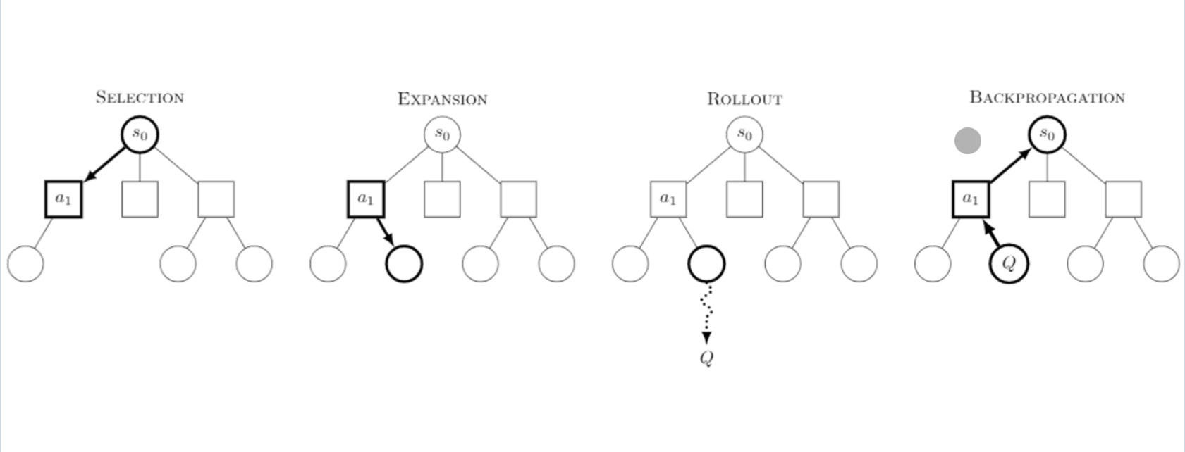

AlphaGo: A case study

The game has a large number of states. The rewards we use are $\plusminus 1$ based on the player won. We define policies for both the players and train the policies with self-play.

Making use of the symmetry of the game, we can use the episodes of the opponent player seen before to train the policy.

AlphaGo used these exact MC methods with neural networks (CNNs, which is super useful for Go) to learn the probabilities and outcome rewards. It was trained with a lot of human games to train initial value networks. The developers also hand-crafted features to represent knowledge in the game.

AlphaZero, an extension of this, relaxed the constraint of requiring a lot of human data and scaled.

All these algorithms have been model-free. That is, we cannot estimate the consequences of our actions in the environment, and are simply learning based off our experiences. We are not learning anything about the dynamics of the environment.

On the flip side, if we know the model of the world, can we do better? So given a world model, how do we use it?

Model-based RL

We learn the model of the world from experiences, and then plan a value function (and/or policy) from the model. What is a model? A representation of an MDP $(S,A,T,R, \gamma)$, and we try to approximate $T, R$.

Assumption. A key assumption that developers make is that the state transitions and rewards are conditionally independent.

We have the experience $S_1, A_1, R_2, \dots, S_T$, and we just train a model in a supervised problem setting $S_i, A_i \to R_{i + 1}, S_{i + 1}$. Learning $R$ is a regression problem and learning $P$ is

How do we use the learned model? Since the learned model has errors and uncertainty, training a policy would take a long time. It is like we are learning the rules of Go whereas previously we knew the rules, and were just trying to win.

The advantages of model-based RL is the it can use all the (self, un) supervised learning tricks to learn from large scale data and can reason about uncertainty. The disadvantage is that we need to first build a model, and then estimate a value from the estimated model - introduced two sources of error.

Introduction to Transformers and Language

A function approximator (neural networks) needs to be good for the task. For example, CNNs were great for Atari and Go but they did not work well for language.

What are the right inductive biases for language then? The attention mechanism was again borrowed from some cognitive functions of the brain. An attention matrix tries to find the alignment of elements within a sequence. Before the scaled dot product attention, there were multiple variants of the formulation -

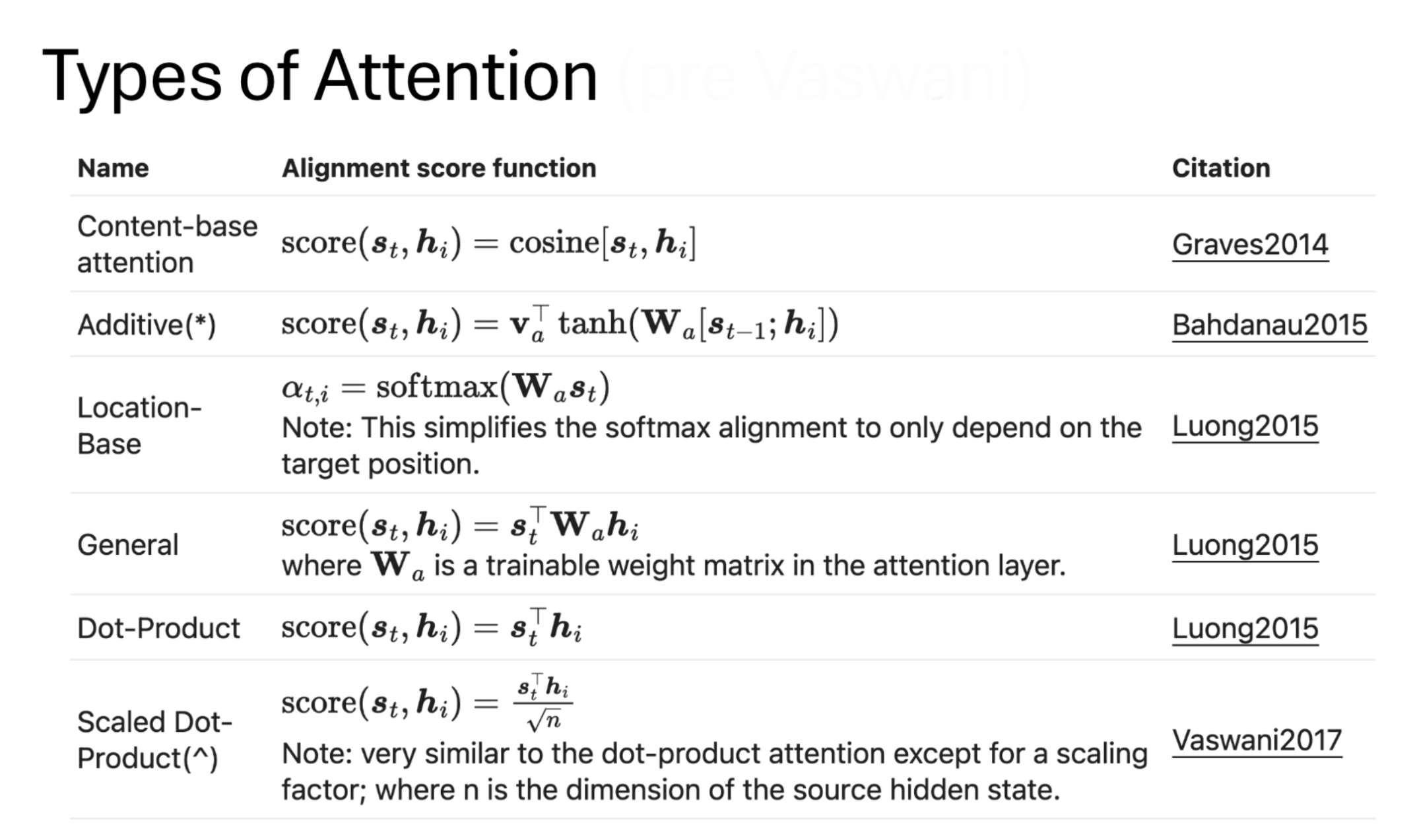Self-attention was first proposed by Cheng et al. in 2016 (originally called intra-attention) that brought in a sense of understanding in models - finding relations between elements of the same sequence.

In 2015, there was a concept of global vs local attention introduced in the form of windowed-attention. This concept is being used widely in vision and language based systems.

Let us discuss the intuition for scaled dot product attention -

Query: What are the things I am looking for?
Key: What are the things I have?
Value: What are the things I will communicate?

So essentially, the queries attend to the keys to find the aligned ones, and the corresponding values are returned. The multi-head part of the architecture is simply the multiple ways of learning these alignments between the query and key sequences. The alternate way of thinking about it is, using an ensemble representation to provide robustness in our predictions. Furthermore, to add a notion of position in the sequence, a positional encoding is added to the sequence elements.

To apply all these mechanisms to language, we need a way to represent language as sequences - this step is known as tokenization. Word-level is too discrete (causes issues for questions like “how many r’s are in ‘strawberry’?”) and character-level is too redundant (often causes issues for questions like “Is 9.9 greater than 9.11?”. The current standard is a sub-word (Tiktoken Byte Pair Encoding BPE) that is learned from a representative subset of data.

The other ideas are to use heuristics for numerical values like new tokenizers and right-to-left processing, etc. The amount of research done in tokenization is underwhelming as compared to the rest of the transformer stack. People have also come up with byte-level transformers and LCMs. Since bytes form too long sequences, people tried hierarchical representations that kind of work. However, there are many training issues with this and byte-encoding issues (PNG and Unicode are weird encodings). They were only able to train a 7B model with the byte-level learning.

Language modeling is another long-standing problem that is a fundamental cornerstone to make these networks learn. The two popular mechanisms used are

Infill (like in BERT): The 47th US President is [??] Trump
Next Token prediction (like in GPT): The sun rises in the ??

RNNs had an encoder-decoder architecture wherein the initial sequence is encoded into a vector (latent space) and it is then decoded into another sequence. This terminology has been carried through and is still used in transformers. The original paper started out as an encoder-decoder architecture, but these models are not used much anymore.

Encoder only models (auto encoding models) - They are used for Sentence classification, NER, extractive question-answering and masked language modeling. Examples are BERT, RoBERTa, distilBERT.
Decoder only models (auto regressive models) - They are used for text generation and causal language modeling. Examples are GPT-2, GPT Nero, GPT-3

Check this repository by Andrej Karpathy for a clean implementation of GPT.

How does all this relate to RL?

We now have a neural net architecture that works well on language. How about using this for MDPs with language-based state-action spaces.

[Paper Discussion] 2xDQN network

As we have seen the Q-learning update

\[Q(S_t, a_t) \gets Q(s_t, a_t) + \alpha[r(s_t, a_t) + \gamma \max_{a’} Q(s’, a’) - Q(s, a)]\]

The problems with Q-learning are

Curse of dimensionality - High dimensions and continuous state spaces do not work
Slow convergence
Inefficient generalization
Exploration-exploitation trade-off

This led to Deep Q-learning. The idea is to replace Q0tables with Neural networks to approximate Q-functions.

*Experience replay stores the agent’s past experiences in a replay buffer. The algorithm randomly samples episodes for training, to break the correlation between consecutive experiences.
Target Networks - Uses a separate, slower updating networking to compute target Q-values. Reduces instability caused by changing Q-values too frequently during learning.

The problems with this are

Overestimation of Q-values - due to the mathematical formulation the Q-values are over-estimated (has been proved mathematically)
Sample inefficient - uses large amount of e
Catastrophic forgetting - may forget previously learned experiences when trained on new experiences

This led to Double Deep Q-learning. They decouple the action evaluation and action selection networks. The online network is used for action selection whereas the action value function evaluates the action. Previously, to stabilize the learning in Q-learning, the updates to action selection network were less frequent leading to choosing sub-optimal actions in some cases.

The problems with this approach are

Might not completely eliminate the overestimation bias - Since action selection and value estimation are not completely decoupled.
Leads to slower convergence in some environments - where overestimation is helpful (high exploration settings)
Sensitive to hyper parameters
Still susceptible to some core DQN issues - Sparse rewards, discrete action space, sample inefficient.

After this, newer methods were proposed such as Rainbow Deep Q-learning - Combination of previous improvements - Prioritized experience replay, uses a dueling network (two explicit specialized networks) for evaluation and selection, Stabilized learning via distributional RL, and Multi-step updates.

RL Agents for LLMs

The typical LLM training pipeline is as follows

SfM fine-tuning - Depends heavily on human expert demo data, and requires a lot of effort. This step can be compared to behavior cloning in RL
Some pipelines also talk about pre-training that can be thought of as weight initialization. This step is not used so much anymore.
After this stage, learning based on feedback, has become a standard step. It comes in many forms, RLHF, RLAIF, etc. The primary approach, Reinforcement Learning with Human Feedback essentially rates different texts generated by the AI, and uses this as a reward model and improves the model considering it as a policy.

This step is cheaper than the other steps, so companies are pushing towards improving this. However, in practice it does not seem to work without pre-training.

This step also involves training a human-proxy reward function. In whole, this is known as post-training development.

RLHF

As we mentioned, the goal is to collect preference feedback and train a reward model. It is a kind of a personalized learning to correct the text generated by the model. One thing to note is that the rewards are given towards the end and there are no intermediate rewards.

For the policy training itself, we have studied value and policy based algorithms. If the value of the MDP is estimated, the policy can be determined implicitly (argmax or epsilon-greedy). However, values and rewards of partial sentences are more difficult to estimate.

Due to these limitations, researchers have gravitated towards policy-based RL. It has better convergence properties and is effective in high-dimensional or continuous actions spaces. However, they can converge to a local optimal rather than a global optima.

“”” I was super sleepy after this, please update after watching the recording “””

Now, for each step, we make a decision within a one-step MDP

Expectation equation
- SFT step is important

Policy Gradient Theorem - For any differential blue policy $$\pi_\theta (s, a)

AI Agents