Automata Notes
Overview
Theory of Computation discusses what can and cannot be done with computers. Moreover, how “hard” or “easy” a given problem is. For instance, consider the problem of determining whether a given multivariate polynomial with integer coefficients has integer roots. This problem is undecidable - we cannot write a deterministic algorithm which halts in finite time that always gives the correct answer for a given polynomial. Through the course, we will explore various techniques and theorems through the course to answer questions like these.
Example. Given a language \(L_1 = \{a^nb^m: n,m \geq 0\}\), decide whether a word is present in this language or not. We will see that such a language can be written using a DFA.
Example. Suppose we have \(L_2 = \{a^nb^n: n \geq 0\}\). Can we construct a DFA for the same?
It can be shown that such a language cannot be represented using a DFA. Instead, we use an instrument known as pushdown automaton.
A pushdown automaton has a stack associated with a DFA. Every transition in the automaton describes an operation such as “push” and “pop” on the stack. A string is accepted by the automaton if the stack is empty at the end of the string. The languages accepted by such automatons are known as context-free grammar.
Example. Extending the previous example, consider the language \(L_3 = \{a^nb^nc^n:n \geq 0\}\). Turns out, a pushdown automaton cannot represent this language.
We have a Turing machine that represents the ultimate computer that can perform any computation (not all). This machine has a ‘tape’ associated with it along with different decisions at each section of the tape. The languages associated with these machines are known as unrestricted grammar.
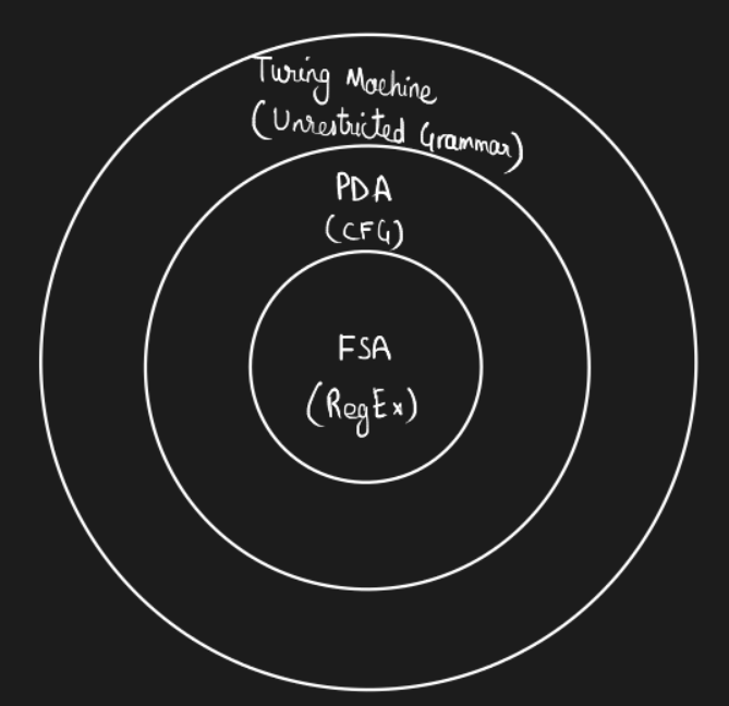
These machines and the associated languages can be represented using a diagram known as Chomsky hierarchy. We will also prove that adding non-determinism affects the expressive power of PDAs but not of DFAs and TMs.
Definition. A finite state automaton is defined as a tuple \((Q, \Sigma, \delta, q_0, F)\), where
- \(Q\) is a finite non-empty set of states,
- \(\Sigma\) is the alphabet with a set of symbols,
- \(\delta: Q \times \delta \to Q\) is the state-transition function,
- \(q_0 \in Q\) is the initial state, and
- \(F \subseteq Q\) is the set of accepting states.
A language \(L\) is a subset of strings over \(\Sigma\), whereas \(\Sigma^*\) represents the set of all possible strings that can be constructed with the alphabet. The \(*\) operator is known as Kleene-star operator representing \(0\) or more repetitions of symbols from an alphabet.
Is the set \(\Sigma^*\) countable?
Example. Let us consider the language \(L_2 = \{a^nb^n:n\geq 0\}\) we saw before. How do we write the context-free grammar for this language? We write a set of base cases and inductive rules as follows -
Typically, we use \(S \to \epsilon\) as the base case. We start out with the string \(S\), and then use the above rules to keep replacing the \(S\) until we obtain a string consisting only of terminals. Here, the symbols \(a, b,\) and \(\epsilon\) are terminals whereas \(S\) is a non-terminal.
Example. Consider the grammar of matched parentheses. This is given by -
Definition. A context-free grammar is defined as a tuple \((V, \Sigma, R, S)\), where
- \(V\) is a set of non-terminals or variables,
- \(\Sigma\) is the alphabet,
- \(R: V \to (V \cup \Sigma)^*\) is the finite set of rules, and
- \(S \in V\) is the start symbol.
The language of a given grammar is the set of all strings derivable using the rules.
Example. Consider the language \(\{a^nb^nc^n: n > 0\}\). This can be represented by the unrestricted grammar as -
These set of rules are very similar to CFG except for the fact that, now, we have strings on the LHS too. Notice how \(A, B\) are used to convey information across the string when new \(a\)’s or \(b\)’s are added.
Homework. Write the unrestricted grammar rules for the language \(L = \{a^{n^2} : n \in \mathbb Z^+\}\)
Definition. An unrestricted grammar is defined as a tuple \((V, \Sigma, R, S)\), where
- \(V\) is a set of non-terminals or variables,
- \(\Sigma\) is the alphabet,
- \(R: (V \cup \Sigma)^* \to (V \cup \Sigma)^*\) is the finite set of rules, and
- \(S \in V\) is the start symbol.
Definition. Regular expressions are defined by the following set of rules -
-
\(\phi, \{\epsilon\}, \{a\}\) (for any \(a \in \Sigma\)) are regular expressions.
-
If \(E_1, E_2\) are regular expressions,
- \(E_1 + E_2\) (union),
- \(E_1E_2\) (concatenation)
- \(E_1^*\) (Kleene star), and
- \((E_1)\) (parenthesis)
are all regular expressions.
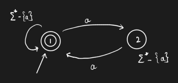
Example. Consider \(L = \{\text{strings with even number of a's}\}\). This can be represented using the regular expression \(b^*(ab^*ab^*)^*\).
Homework. Suppose \(L\) is restricted to have only an odd number of \(b\)’s. How do we write the regular expression for this language?
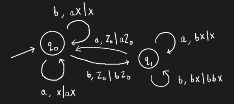
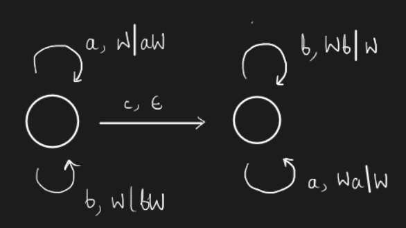
In general, PDAs are represented as a Finite State Machine. That is, we have an action associated with each transition. An empty stack is denoted using the symbol \(Z_0\). That is, the stack begins with a single symbol \(Z_0\). Each transition is represented as \(l, A\), where \(l\) is a letter and \(A\) is an action such as
- \(X \vert aX\) - push
- \(aX \vert X\) - pop
- \(W\vert Wa\) - not sure what this is
Now, a string is rejected by the FSM in two scenarios -
- There is no transition defined at the current state for the current symbol in the string, and
- The stack is not empty, i.e. popping the stack does not yield \(Z_0\) at the end of the string input.
Chomsky Hierarchy
Regular Expressions
We define these languages using a base case and an inductive rule. Empty string is not the same as the empty set. The base case to be considered is \(L = \{\epsilon\}\)?
Inductive Rules
Lemma. If \(E_1, E_2\) are regular expressions, then so are
- \(E_1 + E_2\) - Union
- \(E_1.E_2\) - Concatenation
- \(E_1^*\) - Kleene star
- \((E_1)\) - Parentheses
“Nothing else” is a regular expression. That is, we must use the four rules mentioned above to construct a regular expression.
The fourth rule can be used as follows - \(L((ab)^*) = \{\epsilon, ab, abab, ababab, ...\}\). The parentheses help us group letters from the alphabet to define the language.
Example. Construct a language with only even number of a's'. Good strings include \(\{aba, baabaa\}\), and bad strings include \(\{abb, bbabaa\}\).
The automata can be easily drawn as -
How do we write a regular expression for this? Consider the expression \(R = (ab^*ab^*)^*\). However this expression does not include strings that start with \(b\).
Homework. Try and fix this expression -
\[R = b^*.(ab^*ab^*)^*\]
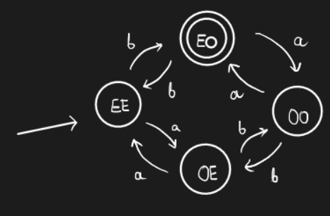
Example. Construct an expression for defining the language \(L = \{\text{all strings with even number of a's} \text{and odd number of b's}\}\)
The following automaton would work for this language -
Homework. Find a regular expression for the above language.
Example. What language does the regular expression \(b^*ab^*(ab^*ab^*)^*\)?
It represents the language with an odd number of \(a\)’s. How do we check this? Start with the base cases - It has \(\epsilon\), and it also has \(\{ab, ba\}\). Try to check the pattern and use induction.
We will soon learn how to derive relations such as “Is \(L = \phi\)?”, “Is \(\|L\| = \infty\)?”, “Is \(L_1 \subset L_2\)?”… All we are doing right now is exploring all the topics in the course using a BFS approach.
Representation of Push-Down Automata
The bottom of the stack contains a special character that indicates the bottom of the stack. We design a Finite State Machine which knows the special characters (for bottom of the stack or other purposes) and also the top element in the stack. This FSM can pop or push on the stack to go to the next state.
Example. Represent \(L = \{a^nb^n\}\) using a FSM.
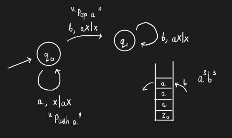
This is how a FSM is represented. A string is accepted iff the stack is empty. Note the transition from \(q_0\) to \(q_1\). It says that the top of the stack must be \(a\). In case it isn’t the case, the string is rejected.
In a FSM, the string is rejected due to one of the two reasons -
- No transition for the given input symbol or we reach the top stack symbol (in the case of finite length languages)
- Input is over, and the stack is not empty.
Example. Try the same for \(L = \{\text{equal \#}a's \text{ and } b's\}\).
Does this work?
Non-determinism
Example. Represent \(L = \{ww^R\} \| w \in (a + b)^*\}\). Here, “R” represents reverse. That is, this language is the language of palindromes. Here, we keep pushing and then we keep popping after a decision point. The decision point is a non-deterministic guess. If there is a correct guess, then the algorithm will work.
Example. Is \(n\) composite? How do we design a non-deterministic algorithm for this problem?
- Guess for a factor \(p < n\)
- Check if \(p\) divides \(n\). If the answer is “yes” then it is composite, else repeat.
How do we reject empty strings in PDA?
Does adding accepting states in the FSM increase the representation power? Does using the special symbol in between the stack increase the representation power?
The reference textbook for this course is “Hopcroft Ullman Motwani.”
Homework. Find the number of binary strings of length 10 with no two consecutive 1’s.
Answer. \(f\) considers bit strings starting with \(0\) and \(g\) considers bit strings starting with \(1\).
\[\begin{align} f(1) &= 1; f(2) = 2; \\ g(1) &= 1; g(2) = 1 \\ f(n) &= f(n - 1) + g(n - 1); \\ g(n) &= f(n - 1); \end{align}\]\(f: \{1, 2, 3, 5, 8, \dots\} \\ g: \{1, 1, 2, 3, 5, \dots \}\) Therefore, there are \(144\) such required strings.
Example. How do we construct an automata which captures the language of binary strings with no two consecutive 1’s? We use something known as a trap state. All the bad strings will be trapped in that state, and no transition from the trap state will lead to a final state. Consider the following automaton.
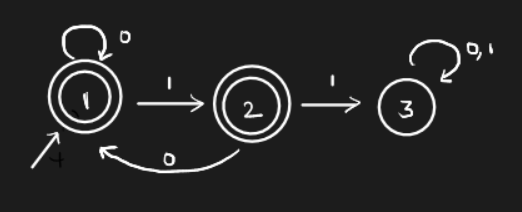
Here, the 3rd state is the trap state.
Extended transition function
\(\hat \delta : Q \times\Sigma^* \to 2^Q\) is defined as
\[\hat \delta(S, aW) = \begin{cases} \delta(S, a) & w = \epsilon \\ \hat \delta(\delta(S, a), W) & \text{otherwise} \end{cases}\]For the sake of convenience we drop the hat and use \(\delta\) for the extended function (polymorphism).
Homework. Read the proof for showing the equivalence of language sets in DFA.
Non-determinism
Non-determinism basically refers to the procedures where we get the same output from the same input through multiple runs. In don’t care non-determinism, we get the same output with different algorithms/procedures. However, in don’t know non-determinism, a single stochastic algorithm goes through many runs (scenarios) to get the answer.
A deterministic automaton has a single choice of transition from a given state for a given symbol from the alphabet. However, in the case of a non-deterministic automata, such guarantee does not exist. The next state for a given symbol from a given state of the NFA is a set of states rather than a single state. There are two types of NFA as discussed previously.
- Don’t know NFA - Guess the right choice
- Don’t care NFA - All choices give the same result
One might ponder if NFAs are more expressive than DFAs. The answer is surprisingly no. Non-determinism can be introduced to an automaton in two ways -
- Choice of subset of states for each transition
- \(\epsilon\)-transitions
Example. Construct an automaton to represent the language \(L = \{abc\} \cup \{\text{all strings ending in b}\}\) whose alphabet is \(\{a,b,c\}\)
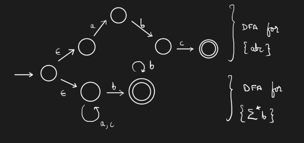
Note. We have introduced \(\epsilon\)-transitions in this automaton.
As we shall see later in the course, the three models - DFA, NFA, and NFA with \(\epsilon\)-transitions; are all equivalent in terms of expressive power.
Properties of Languages
We mainly check two properties of languages - decision and closure.
-
Decision - Is \(w \in L\)? (Membership Problem) - decidable for regular languages.
Decidable problems - Problems for which we can write a sound algorithm which halts in finite time.
We can also consider problems like - Given \(DFA(M_1)\) and \(DFA(M_2)\), Is \(L(M_1) = L(M_2)\)? or \(L(M_1) \subset L(M_2)\)?
Is \(L = \phi\)? Is \(L\) finite? Is \(L\) finite and has an even number of strings? We can also ask questions about the DFA - Can \(L(M)\) be accepted by a DFA with \(k < n\) states (minimalism)?
Example. Can we build a DFA whose language is \(L = \{\text{bit strings divisible by } 7\}\) with less than 7 states? Turns out, the answer is no.
Finally, we can ask a very difficult question such as - Show \(L\) cannot be accepted by any DFA. The technique for solving such a question is known as the Pumping Lemma. This lemma is based on the Pigeonhole principle.
-
Closure - closure using Union, Intersection, Kleene Star, and Concatenation. The question we ask is if \(L_1, L_2\) belong to class \(C\), then does \(L_1 \texttt { op } L_2\) belong to \(C\)?
We plan to show the equivalence of the following models -
- DFAs
- NFAs
- NFA-\(\epsilon\)
- Regular Expressions
Homework. Draw a DFA for the language \(L_1 \cup L_2\) where \(L_1\) is \(a\) followed by even number of \(b\)s and \(L_2\) is \(a\) followed by odd number of \(c\)s.
Regular Expressions
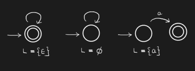
They are defined using base cases and inductive cases. Before we discuss this, we define closed-world assumption. It is the presumption that a statement that is true is also known to be true. Therefore, conversely, what is not currently known to be true, is false. More info regarding this topic can be found here. The base cases for regular expressions are given as follows.
\[\begin{align} L(a) &= \{a\} \\ L(\epsilon) &= \{\epsilon\} \\ L(\phi) &= \phi \text{ (An empty set)} \end{align}\]The inductive cases are
\[\begin{align} L_1, L_2 &\to L_1 \cup L_2 \\ L_1, L_2 &\to \{uv \vert u \in L_1, v \in L_2\} \\ L &\to L_1^* \end{align}\]RE \(\equiv\) NFA-\(\epsilon\)
To begin with, we convert the base cases of regular expressions to NFA-\(\epsilon\)s. Here are the automatons
Now, for the inductive cases -
-
For union of \(L_1\) and \(L_2\), consider the NFAs of both languages. Create a new start state \(s\) and final state \(f\). Connect \(s\) to the start states of both NFAs with \(\epsilon\) transitions and the final states of both NFAs to \(f\) with the same transitions.
How do we prove that this construction represents the union?
-
For concatenation of \(L_1\) and \(L_2\), connect all the final states of \(L_1\)’s NFA to all the start states of \(L_2\)’s NFA using \(\epsilon\) transitions.
-
For \(L^*\), connect all the final states of the NFA to the start states of the NFA using \(\epsilon\) transitions. However, this does not accept \(\epsilon\). Fix it. Think.
Decision Properties
Membership Problem
Does \(w \in L\)? How do we show that this problem is decidable? The algorithm is well-known.
Emptiness Problem
Is \(L(M) = \phi\)? This problem can be solved using reachability in graphs. One can check if the final states are reachable from the start state. It can be achieved using fixed point. This method is essentially propagating the frontier from the start state. We add neighbors of all the states in the current frontier and keep expanding it. We do this until our frontier does not change. This frontier is the fixed point.
Infiniteness Problem
Is \(L(M)\) finite? We need to search for a loop in the graph to answer this question. Suppose our DFA has \(N\) states. If the DFA accepts a string whose length is greater than or equal to \(N\), then a state has to repeat while forming this string. This observation is a result of the Pigeonhole principle.
This check is both necessary and sufficient. If a language is infinite, then it means that it has a string of length greater than \(N\). How are we going to use this property to check the infiniteness of the language? Is there a decidable algorithm?
Claim. If there is a string of length \(\geq N\) in \(L\), then there is a string of length between \(N\) and \(2N - 1\). Think about the proof. Clue. You can use at the most \(N - 1\) self loops.
It is sufficient to test for the membership of all strings of length between \(N\) and \(2N - 1\).
Pumping Lemma
Problem. Show that \(L = \{a^nb^n\}\) is not regular.
We use proof by contradiction. Assume that a \(DFA(M)\) with \(N\) states accepts \(L\).
Theorem. Pumping Lemma. For every regular language \(L\), there exists an integer \(n\) , called the pumping length, where every string \(w \in L\) of length \(\geq n\) can be written as \(w = xyz\) where
\[\begin{align} \vert xy \vert &\leq n \\ \vert y\vert &> 0\\ \forall i \geq 0,\ & x(y)^iz \in L \end{align}\]Let us understand this by proving \(L = \{a^nb^n \vert n > 0\}\) is not regular using contradiction. Assume there is a \(DFA(M)\) with \(N\) states that accepts \(L\).
Now, consider the string \(a^Nb^N\). Now, define \(a^n\) as \(xy\). Let \(x = a^j\) and \(y = a^k\) where \(n \leq N\). According to the pumping lemma, \(a^j(a^k)^ib^N \in L\). Therefore, there can’t exist a DFA that represents \(L\).
Homework. Prove that the language with equal number of \(a\)‘s and \(b\)’s is not regular.
The idea is to use closure properties.
Homework. Prove the pumping lemma.
Answer. Consider a DFA\((Q, \Sigma, Q_0, \delta, F)\) with \(N\) states, and a word \(w\) such that \(\vert w \vert = T \geq N\) belongs to \(L\). Now, let \((S_i)_{i =0}^T\) (0 - indexed) be the sequence of states traversed by \(w\). The state \(S_L\) is an accepting state as \(w \in L\). Also, there exist \(0 \leq i < j \leq N\) such that \(S_i = S_j\) as there are only \(N\) states in the DFA (Pigeonhole principle). Now, define the string formed by \(S_0, \dots, S_i\) as \(x\), the one formed by \(S_i, \dots, S_j\) as y, and that formed by \(S_j, \dots, S_T\) as \(z\). We have \(w = xyz\). Also, \(\vert y \vert > 0\) as \(i < j\) and \(\vert xy \vert \leq N\) as \(j \leq N\).
Since \(S_i = S_j\), we can pump the string \(y\) as many times as we wish by traversing cycle \(S_i, \dots, S_j\). Now, since \(S_T \in F\), the string formed by the sequence \(S_0, \dots, \{S_i, \dots, S_j\}^t, \dots, S_T\) (\(t \geq 0\)) also belongs to \(L\). This word is equivalent to \(xy^iz\). \(\blacksquare\)
NFA \(\equiv\) DFA
We convert a NFA to DFA using subset construction. That is, if \(Q\) is the set of states in the NFA, then \(2^Q\) will the set of states in the DFA. Initially, we construct the start states using the subset of start states in the NFA. Then, we build the following states in the DFA by tracing all the states reached by each character in the NFA into a single subset. If any of the subset consists of a final state, then that subset state is made into a final state in the DFA.
This equivalence can also be extended to show the equivalence of NFA-\(\epsilon\) and \(DFA\).
DFA Minimization
All DFAs with minimal number of states are isomorphic.
Distinguishable states
Consider a DFA \((Q, \Sigma, Q_0, \delta, F)\). States \(q_i,q_j \in Q\) are said to be distinguishable iff there exists a word \(w \in \Sigma^*\) such that \(\delta(q_1, w) \not \in F\) and \(\delta(q_2, w) \in F\) or vice versa.
One can merge indistinguishable states to minimize a DFA.
Context-Free Grammar
Let us try to write the grammar for the language \(L = \{a^ib^jc^k \vert i = j \text{ or } j = k\}\). Consider the following rules
\[\begin{align} S &\to S_1 \vert S_2 \\ S_1 &\to aS_1bC \vert C \\ S_2 &\to AbS_2c \vert \epsilon \\ C &\to cC \vert \epsilon \\ A &\to aA \vert \epsilon \end{align}\]In general, union is straightforward to write in CFG due to rules like rule 1. However, there is an ambiguity in the above rules. For example, the word \(a^3b^3c^3\) can be generated using different derivations. We’ll discuss this later in the course.
As we discussed before, a context free grammar \(G\) is defined by \((V, \Sigma, R, S)\). A string is accepted by the grammar if \(w \in \Sigma^*\) and \(R \xrightarrow{*} w\). That is, the rules must be able to derive \(w\).
A one-step derivation is given by \(u_1Au_2 \to u_1\beta u_2\) if \(A \to \beta \in R\) and \(u_1, u_2 \in (V \cup \Sigma)^*\).
Consider the set of rules for defining arithmetic expressions. The language is defined over \(\Sigma = \{+, -, \times, \div, x, y, z, \dots\}\).
\[\begin{align} S &\to x \vert y \vert z \\ S &\to S + S \\ S &\to S - S \\ S &\to S \times S \\ S &\to S \div S \\ S &\to (S) \end{align}\]Now, for an expression such \(x + y \times z\), we can give a left-most derivation or a right-most derivation. A precedence order removes ambiguities in the derivation. In programming languages, a parser removes these ambiguities using some conventions.
Homework. Try and write the set of rules for the language which consists of \(a\)s and \(b\)s such that every string has twice the number of \(a\)s as that of \(b\)s.
Answer. We try to write the rules for equal number of a’s and b’s, and try to extend them.
\[\begin{align} S &\to \epsilon \\ S &\to aSb \ \vert \ Sab \ \vert \ abS \\ S &\to bSa \ \vert \ Sba \ \vert \ baS \end{align}\]Does this work?
Note. \(\vert R \vert\) is finite.
We had seen the CFG for the language \(L = \{a^nb^n\}\). How can one prove that the rules represent that language? That is, how do we know that the rules generate all the strings in the language and no other strings?
Consider the language we saw in the previous lecture - strings with equal number of a’s and b’s. The possible set of rules are -
\[\begin{align} S &\to aB \ \vert \ bA \\ B &\to b \ \vert \ bS \ \vert \ aBB \\ A &\to a \ \vert \ aS \ \vert \ bAA \\ \end{align}\]The thinking is as follows -
- \(S\) generates strings with equal number of a’s and b’s. \(B\) generates strings with one more b than a’s, and similarly for \(A\).
- To write the inductive cases of \(S\), we consider strings starting with both a and b. Inductive cases for \(A, B\) are also constructed similarly.
Another possible set of rules are -
\[\begin{align} S &\to aSb \ \vert \ bSa \\ S &\to \epsilon \\ S &\to SS \\ \end{align}\]These rules are the minimized set of the rules I wrote for the hw in the last lecture.
Grammars
We can write grammars in canonical forms. A grammar is said to be in Chomsky normal form if the rules are of the form
\[\begin{align} C \to DE &\text{ - one non-terminal replaced by 2 non-terminals} \\ C \to a &\text{ - one terminal replaced by a terminal} \end{align}\]Claim. Any grammar \(G\) (\(\epsilon \not\in L(G)\)) can be converted to an equivalent Chomsky Normal form.
Another canonical form of grammar is Greibach normal form. The rules are of the form
\[\begin{align} C &\to a\alpha \end{align}\]Each non-terminal converts to a terminal followed by a symbol in \((V \cup \Sigma)^*\). Similar to the Chomsky form, every grammar can be converted to the Greibach normal form.
Push Down Automatons
Consider the language \(L = \{wcw^R \vert w \in (a + b)^*\}\).
Aside. Try writing the Chomsky normal form rules for the above language. \(\begin{align} S &\to AA_0 \mid BB_0 \mid c \\ A_0 &\to SA \\ B_0 &\to SB \\ A &\to a \\ B &\to b \\ \end{align}\)
The pushdown automaton for this language is given by -
How do we take a grammar and produce the normal form of the grammar? We shall learn techniques such as eliminating useless symbols, elimination epsilon and unit productions. These will be used to get the designable form of the grammar that can also be used to show languages which are context-free using the pumping lemma.
The notation \(\alpha_1 \xrightarrow{n} \alpha_2\) is used to denote that \(\alpha_2\) can be derived from \(\alpha_1\) in \(n\) steps. The \(*\) over the arrow represents the derivative closure of the rules.
Grammars \(G_1, G_2\) are equivalent iff \(L(G_1) = L(G_2)\). For example, we have seen two grammars for the language \(L = \text{ strings with } \#a = \#b\), and they are both equivalent.
Derivation trees
- Trees whose all roots are labeled.
- The root of the tree is labeled with the start symbol of the grammar \(S\).
- Suppose A is the label of some internal node, then A has a children \(X_1, \dots X_R\) iff \(A \to X_1\dots X_R \in R\).
- \(\epsilon\) can only be the label of leaf nodes.
Derivations
Grammars with multiple derivation trees are ambiguous. Are there languages for which any grammar is ambiguous? Such languages are called as inherently ambiguous.
Homework. Find examples of inherently ambiguous grammars.
Simplifying grammars
Definition. A variable \(B\) is productive in \(G\) iff \(B \xrightarrow[G]{*} w\) for some \(w \in \Sigma^*\).
Definition. A variable \(B\) is reachable from the start symbol \(S\) of \(G\) if \(S \xrightarrow[G]{*} \alpha B \beta\) for some \(\alpha, \beta \in (\Sigma \cup V)^*\).
We useful variable \(X\) is productive and reachable. These are necessary conditions but not sufficient. For example, consider the following grammar.
S -> AB
A -> c
Here, \(A\) is useless even if it is productive and reachable.
Definition. A variable \(X\) is useless if there is no derivation tree that gives \(w \in \Sigma^*\) from \(S\) with \(X\) as the label of some internal node.
Fixed point algorithm
The idea is to find a monotonic algorithm which gives us the set of useful symbols at the fixed point of the underlying function.
Firstly, let us try this for productive variables. We propose the following algorithm.
\[\begin{align} P_0 &= \phi \\ P_i &\to P_{i + 1} \\ &\triangleq P_i \cup \{N \mid N \to \alpha \in R \text{ and } \alpha \in (\Sigma \cup P_i)^* \} \end{align}\]For example, consider the grammar
S -> AB | AA
A -> a
B -> bB
-- The algorithm
P_o = \phi
P_1 = {A} // Rule 2
P_2 = {A, S} // Rule 1
P_3 = {A, S}
Therefore, the symbols \(S, A\) are productive in the above grammar. We propose a similar algorithm for reachable states in the grammar.
\[\begin{align} R_0 &= \phi \\ R_i &\to R_{i + 1} \\ &\triangleq R_i \cup \{P \mid Q \to \alpha P \beta; \alpha, \beta \in (\Sigma \cup P_i)^* \text{ and } Q \in R_i\} \end{align}\]Definition. A nullable symbol is a symbol which can derive \(\epsilon\). These symbols can be eliminated.
Definition. A unit production is a rule of the form \(A \to B\) where \(A, B \in V\).
We shall continue discussing simplifying grammars. As an initial step, we can get rid of symbols which are either unreachable or unproductive. However, the order in which we check productivity and reachability affects how the grammar is simplified. For example, consider the grammar
S -> a
S -> AB
A -> a
Now, if we eliminate unreachable symbols first (that is none), and then eliminate unproductive symbols (\(B\)), we get
S -> a
A -> a
Notice that the above simplified grammar has a redundant rule. However, if we check for productivity (\(B\) is eliminated) and then reachability (\(A\) is unreachable), we get
S -> a
Claim. Eliminating unproductive symbols followed by unreachable symbols gives a grammar without any useless variables.
Homework. Prove the above claim.
\(\epsilon\)-productions
Suppose \(G\) is a CFG such that \(L(G)\) has \(\epsilon\), then \(L(G) - \{\epsilon\}\) can be generated by a CFG \(G_1\) which has no \(\epsilon\)-productions (rules of the form \(A \to \epsilon\)).
Nullable symbols
\(A\) is nullable if \(A \xrightarrow[G]{*} \epsilon\).
How do we remove nullable symbols? We can’t just take out a rule of the form \(A \to \epsilon\) as it may make \(A\) unproductive. The way to go about this is to replace each rule of the form \(A \to X_1\dots X_n\) to \(A \to \alpha_1 \dots \alpha_n\) where
\[\alpha_ i = \begin{cases} X_i & X_i\text{ is not nullable}\\ \epsilon &\text{otherwise} \end{cases}\]However, one must be cautious about replacing all the symbols by \(\epsilon\) and also about recursive rules. For instance, consider the following grammar
\[S \to \epsilon \mid aSb \mid bSa \mid SS\]Now, \(S\) is nullable but we can’t replace \(S \to aSb\) by \(S \to ab\) simply. We also need to have the rule \(S \to aSb\) in place for recursion. Basically, for each rule of the form \(A \to X_1\dots X_n\), we need to have all the rules of the form \(A \to \alpha\) where \(\alpha\) spans over all subsets of \(X_1 \dots X_n\).
Unit Productions
To remove unit productions, let us assume that there are no \(\epsilon\)-productions and useless symbols. Now, we need to find all pairs \((X, Y)\) such that \(X \xrightarrow[G]{*} Y\). Once we find such pairs, we can try and eliminate the unit symbols themselves, or solely the rules.
Let us take the following grammar for \(L \{w \mid n_a(w) = n_b(w)\}\)
\[S \to \epsilon \mid aSb \mid bSa \mid SS \\ \text{ simplified to } \\ S \to abS \mid bSa \mid SS \mid ab \mid ba\]and
\[S \to \epsilon \\ S \to aB \mid bA \\ B \to b \mid bS \mid aBB \\ A \to a \mid aS \mid bAA \\ \text{ simplified by just removing } S \to \epsilon\\\]To convert the grammar into Chomsky normal form, we do approximately the following - we replace each rule of the form \(A \to X_1 \dots X_n\) with \(A \to X_1B\) and \(B \to X_2 \dots X_n\). We keep repeating this until there is only a single terminal symbol on the rhs, or two non-terminals.
Consider a grammar in Chomsky form. The derivation tree will consist of nodes with either 2 children (\(A \to BC\)), 1 child (\(A \to a\)) or leaf nodes.
Let the longest path in the derivation tree be \(k\). Then, the upper bound on the length of the word formed is \(2^{k - 1}\) and lower bound is \(k\). Note. The variables from \(V\) can repeat across a path.
Pumping Lemma for CFG
For any CFL \(L\), the language \(L - \{\epsilon \}\) has a Chomsky Normal form grammar.
Theorem. Pumping Lemma For every CFL \(L\), there is a \(n\) such that for all strings \(\vert z \vert \geq n\) with \(z \in L(G)\), there are strings \(u, v, w, x, y\) such that \(z = uvwxy\) and
- \[\vert vwx \vert \leq n\]
- \[\vert vx \vert \geq 1\]
- for all \(z_i = u v^iwx^iy\), \(i \geq 0\), \(z_i \in L(G)\).
It is easy to show \(L = \{a^nb^nc^n \mid n \geq 1\}\) is not a CFL using the above lemma.
Proof of the lemma
If there is a \(z \in L(G)\) such \(\vert z \vert \geq n = 2^k\), then there must be a path of length at least \(k + 1\). Now, due to pigeonhole principle, a variable must repeat in this path in the derivation tree of \(z\).
Now, consider the path \(S, \dots, A, \dots, A, \dots, a\).
- It is easy to the see that the word formed by the subtree below the first \(A\) has length \(\leq n\).
- Also, as there are 2 \(A\)s in the path, the number of letters in the “left” subtree and “right” subtree would be greater than 1.
- These “left” and “right” subtrees can be derived an arbitrary number of times as \(A\) can be derived from \(A\).
Note. To draw some more intuition, call the subtree formed by the first \(A\) as \(T_1\), and the subtree formed by the second \(A\) as \(T_2\). We shall label the word formed by \(T_2\) as \(w\), and the word labeled by \(T_1\) as \(vwx\). Now, \(\vert vx \vert \geq 1\). Think. The “left” and “right” subtree in the above explanation together are formed by the set \(T_1 \setminus T_2\).
Homework. Show that the following languages cannot be represented by CFG.
- \[L = \{a^ib^ic^i \mid j \geq i\}\]
- \[L = \{a^ib^jc^k \mid i \leq i \leq k\}\]
- \[L = \{a^ib^jc^id^j \mid i, j \geq 1\}\]
We shall see that 2 stacks PDA is the most expressive Turing machine.
Can’t there be useless symbols in normal forms? yes -> \(S \to AB\)
Ogden’s Lemma
This lemma is a generalization of pumping lemma. Consider the pumping lemma for the FSA. It basically said that some state must repeat for a string of length \(\geq n\) in the language. Ogden’s lemma talks about a similar claim for CFGs. It will be formally discussed in the next lecture.
Closure properties
The union, concatenation and Kleene closure of CFGs are also CFGs. Proof is left as a homework.
Intersection is not context-free!
Pushdown Automata
Consider the languages \(L_1 = \{wcw^R \mid w \in (0 + 1)^* \}\) and \(L_3 = \{ww^R \mid w \in (0 + 1)^* \}\). Let us build PDAs for these two models.
The stack of the PDA uses different symbols that those from \(\Sigma\). We shall denote the superset of symbols of stack by \(T\). Each transition in the PDA depends on the input symbol and the symbol on the top of the stack. These are similar to the FSA transition diagram. If both of these symbols are satisfied for the transition, we perform an action on the stack by pushing or popping symbols. Note that we can also choose to not perform any action.
We shall also use the symbol \(X\) to denote ‘matching any character’ for the symbols on stack. We can also have \(\epsilon\) transitions in non-deterministic PDAs. \(\epsilon\) transitions basically denote ignoring input symbols.
Note. We can push multiple symbols in each transition but we can only pop one symbol in each transition.
The PDA for \(L_1\) is given by
\[\begin{align} \delta(q_1, c, X) &= (q_2, X) \\ \delta(q_1, 1, X) &= (q_1, GX) \\ \delta(q_1, 0, X) &= (q_1, BX)\\ \delta(q_2, 0, B) &= (q_2, \epsilon) \\ \delta(q_2, 1, G) &= (q_2, \epsilon) \\ \delta(q_2, \epsilon, Z_0) &= (q_2, \epsilon) \\ \end{align}\]The PDA for \(L_3\) is similar but we cannot express this language without non-determinism. We can’t guess where the “middle of the string” occurs without guessing. Therefore, non-deterministic PDAs are more expressive than deterministic ones.
Remember that the non-deterministic PDA accepts a string if there is at least one run that accepts it.
Formal definition of PDA
A Pushdown automata is formally given by the 7 element tuple \(M \lang Q, \Sigma, \Tau, \delta, q_0, Z_0, F \rang\) where
- \(\Tau\) is the set of stack symbols
- \(Z_0\) is a special symbol denoting the bottom of the stack
- \(F\) is the set of final states of the automata
- \(\delta: Q \times (\Sigma \cup \epsilon) \times \Tau \to (Q, \lambda)\) where \(\lambda \in \Tau^*\) is an action performed on the transition.
A string is accepted if one of the runs ends with an empty stack or at a final state. That is, \(L(M) = \{w \mid (q_0, w, Z_0) \vdash^*_M (p, \epsilon, \epsilon)\} \cup \{ w \mid (q_0, w, Z_0) \vdash^*_M (q, \epsilon, \lambda), q \in F\}\). In the following lectures, we shall prove DPDA \(\neq\) NPDA, ‘accepting by empty stack’ \(\equiv\) ‘accepting by final state’ and PDA (NPDA) \(=\) CFG.
We define a move or an arrow as a transition in the PDA.
Instantaneous Description refers to the property of defining a system using a single number. In case of a PDA, the description is given by a numerical representation of (Current string, Remaining input tape, Stack content). These values, that constitute the dynamic information of a PDA, keep changing during moves. The notation \(ID_1 \vdash_M ID_2\) denotes a single transition in the PDA. The notation \(ID_1 \vdash^*_M ID_2\) is a sequence of 0 or more moves.
We have seen the accept criteria in the last lecture. We will show that a PDA built on the final state accept criteria has an equivalent PDA built on the empty state accept criteria.
Greibach Normal Form
CFGs of the form \(A \to a\alpha\).
Note. \(\alpha\) in the above expression consists of non-terminals only!
What are the challenges involved in converting a grammar to a Greibach normal form? It involves the following steps.
Elimination of productions
Suppose we want to remove the rule \(A \to \alpha_1 B \alpha_2\) and keep the language of the CFG same. Then, we consider all rules of the form \(B \to \beta\) and replace each of them by \(A \to \alpha_1 \beta \alpha_2\). After doing this, we can delete the initial production involving \(A\).
Left Recursion
Suppose we have rules of the form \(A \to A\alpha_1 \mid A\alpha_2 \mid \dots \mid A\alpha_r\) which we wish to remove. Now, there would be other rules involving \(A\) of the form \(A \to \beta_1 \mid \dots \mid \beta_s\).
Now, we define a new variable \(B \not\in V\). Then, we write rules of the form \(A \to \beta_1B \mid \dots \mid \ \beta_s B\) and \(\beta \to \alpha_1 B \mid \dots \mid \alpha_r B\). We can then remove all the left-recursive productions of \(A\). Basically, we have replaced left-recursion rules with right-recursion rules.
Ordering of Variables
Simplify the variables in one order? Wasn’t taught?
Equivalence of PDA and CFG
Given any CFG \(G\), we convert it into Greibach normal form. Then, we choose the non-terminals as the stack symbols. The initial symbol in the grammar is taken as the top symbol of the stack initially. For each rule \(A \to a\alpha\) we write the transition \(\delta(q, a, A) = (q’, \alpha)\). We start with a single state in the DFA, and write all the rules on this state. Through this intuition, we have shown that every CFG has a corresponding PDA. Then, we need to show that every PDA has a corresponding CFG.
To show that CFG \(\subseteq\) PDA, we need to show the equivalence of a language in both directions. That is, for every string accepted by the CFG, we need to show that the PDA also accepts it and vice versa. Note that we also have to prove PDA \(\subseteq\) CFG.
## Ogden’s Lemma revisited
Suppose we had to prove the language \(L = \{a^ib^jc^kd^l \mid i = 0 \text{ or } j = k = l\}\) is not CFG. Can we do this using pumping lemma? No. Think.
We do this using Ogden’s lemma which goes something like this. You can give a \(z = z_1 \dots z_m\) such that \(m \geq n\). Now, we can mark positions by choosing a subset of \(z_i\)’s. Then, the \(vwx\) from the pumping lemma must have at most \(n\) marked positions and \(vx\) has at least one marked position. This is a stronger condition as compared to the pumping lemma.
Homework. Show that \(L = \{a^ib^jc^k \mid i \neq j, j \neq k, i \neq k\}\) is not context-free using Ogden’s lemma.
Closure properties of CFLs
- Union - \(L(G_1) \cup L(G_2)\) regular? Yes. Add a rule \(S \to S_1 \mid S_2\).
- Kleene closure - \((L(G_1))^*\) regular? Yes. Add a rule \(S \to S_1S \mid \epsilon\).
- Concatenation - \(L(G_1). L(G_2)\) regular? Yes. Add a rule \(S \to S_1 S_2\).
- Intersection - Consider the example \(L_1 = \{a^ib^ic^j \mid i, j \geq 1\}\) and \(L_2 = \{a^ib^jc^i \mid i, j \geq 1\}\). Both of them are context free but their intersection is not.
- Complement - Easy to show from intersection.
Decision properties of CFLs
Is the language empty?
This is easy to check. Remove useless symbols and show that \(S\) is useful.
Is the language finite?
Consider the Chomsky normal form of the grammar. Draw a graph corresponding to the grammar such that every node has a single edge directed to a terminal or two edges directed to non-terminals.
Claim. If the graph has a cycle, then the language formed by the grammar is infinite. This is intuitive.
We can find cycles using DFS simply.We can derive more efficient methods which is not the goal of this course.
Does a string belong to the language?
The first approach is the following. Get the Greibach form of the grammar. Now, for each letter \(c\) in the string check whether there are rules of the form \(A \to c\alpha\). We consider the values of all such \(\alpha\)s and continue parsing the rest of the input string. Therefore, at each letter in the string we limit the number of possible derivations. If we reach the end of the string without running out of possible derivations at each letter, then the string belongs to the language. Remember that we will start with the start symbol for the beginning of the string.
However, we can see that this method is not very efficient. We shall see the CYK algorithm which works in \(\mathcal O(n^3)\).
Additional closure properties of CFLs
-
\(L(G) \cap R\), where \(R\) is a regular language, is also context-free.
How do we show that \(L = \{ww \mid w \in (a + b)^*\}\) is not context free? It can be shown via pumping lemma which is complicated. However, it is very easy to prove it using the above property.
How do we prove the closure property? Consider a \(PDA(M_1)\) for \(L(G)\) and \(DFA(M_2)\) for \(R\). Now, we construct a ‘product’ PDA similar to what we did in NFAs. We use the ‘final state’ accept PDA for the purpose. The final states would be \(F_1 \times F_2\). It is easy to see that we can get the required property.
CYK algorithm
The Cocke-Younger-Kasami algorithm can be used to check if a string \(w\) belongs to \(L(G)\).
Suppose there is a \(w = w_1 w_2 \dots w_i \dots w_l \dots w_n\) whose membership we need to check. We consider subproblems of the form: Is \(w_{ij} \triangleq w_i \dots w_{i + j - 1}\) derivable from any non-terminal in the grammar? Then, finally, we need to answer is \(w_{1n}\) can be derived from \(S\).
We consider the Chomsky normal form of the grammar for this algorithm. All strings of the form \(w_{j1}\) can be checked easily. For each \(w_{i1}\) we store all the non-terminals that can derive it. Now, the recursion for all \(j \geq 2\) is given by
\[f(w_{in}) = \bigcup_{j = 1}^{n - 1}\bigcup_{A \in f(w_{ij})} \bigcup_{B \in f(w_{i(n - j)})} \{C \mid (C \to AB) \in G \}\]See the following example using the CYK algorithm.
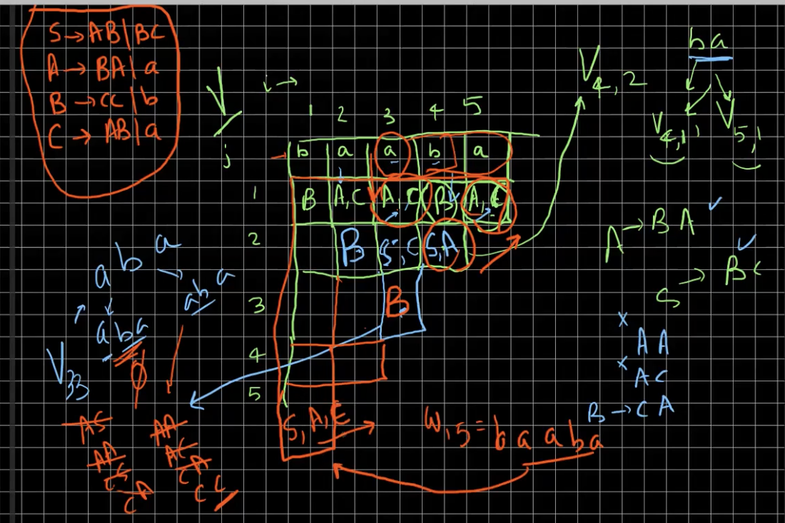
It is easy to see that this algorithm takes \(\mathcal O(n^3)\).
\(\epsilon\) closure
We define \(\epsilon\) closure for a state \(q\) in a DFA as all the states that \(q\) can reach via \(\epsilon\) transitions. Then, to remove all the \(\epsilon\) transitions from \(q\), we add a transition corresponding to all transitions from \(q\) to each of the states in the \(\epsilon\) closure of \(q\). Also, if any state in the \(\epsilon\) closure of \(q\) is final, then \(q\) can also be made as a final state.
Note. Minimal DFAs need not be unique. They are isomorphic.
Satan-Cantor Game
The game goes like this. Satan chooses a random natural number and asks Cantor to guess the number. Cantor gets a chance to guess once on each day. If Cantor guesses the right number, then he can go to heaven. Does Cantor have a strategy that will guarantee him going to heaven? Yes, Cantor can choose numbers in the sequence \(1, 2, 3, \dots\) and eventually it is guaranteed that Cantor chooses the correct number.
Suppose, Satan changes the game by choosing a random integer. Does Cantor have a strategy then? Yes, choose numbers of the form \(0, 1, -1, 2, -2, \dots\). Now, suppose Satan chooses a pair of integers, then how do we get a strategy? We can order the points based on the distance from the origin in the 2D Cartesian plane (Cantor’s pairing function). Similarly, a tuple of \(n\) integers is also enumerable.
Can we give a set for Satan such that the elements are not enumerable? What if Satan chooses \((n_1, \dots, n_k)\) where \(k\) is not known to Cantor. Can Cantor win in this case? Yes. Proof is homework.
Satan can choose the set of real numbers, and in that scenario Cantor would not be able to win. The key idea here is Cantor’s diagonalization argument.
Also, look up Kolmogorov complexity. Enumerability \(\equiv\) Countability.
Enumerability in Languages
A language which is finite will be regular, and we can build an FSA for it. How about infinite languages? CFLs can represent a subset of these languages.
If we categorise the infinite languages as languages which are recursively enumerable and uncountable. Can we build models for recursively enumerable languages?
Turing Machines
Turing wanted to build a machine that could recognize any enumerable language. The inspiration is drawn from the recursive function theory developed by Alonzo Church. There are other people who developed Type-0 grammars which are similar to CFGs but the left hand side of the rules can consist of a string composed of terminals and non-terminals making it context-dependent.
Church and Turing came up with a thesis, and they proposed that Church’s theory and Turing’s machine can be used to compute any effectively computable function.
Aside. Aren’t all languages enumerable with alphabet being a finite set?
“Is \(L(G)\) empty?” is a decidable problem. However, “Is the complement of \(L(G)\) empty?” is not decidable! This property was proven by Godel.
We shall now introduce the notion of Turing machines. Instead of a stack, we have an input tape with a fixed left end. A string is written in the tape with each letter being in a cell of the tape. The machine also involves a control which is essentially a FSM that takes the input from the tape, and performs actions on it. Basically, in PDAs, we could only see the top of the stack, but here we are able to freely traverse over the tape.
Definitions from set theory
Definition. Enumerable of a set refers to the property of being able to define a one-to-one correspondence from the elements of the set to positive integers.
Definition. In computability theory, a set \(S\) of natural numbers is called computably enumerable, recursively enumerable, semi-decidable, partially decidable, listable, provable or Turing-recognisable if
- there is an algorithm such that the set of input numbers for which the algorithm halts is exactly \(S\).
- or equivalently, there is an algorithm that enumerates the members of \(S\). That means that its output is simply a list of all the members of \(S = \{s_1, s_2, s_3, \dots\}\) . If \(S\) is infinite, this algorithm will run forever.
Dovetailing
In the Satan-Cantor game, the idea was to enumerate all possible answers “fairly”.
Let us consider the scenario where Satan chooses a \(k\) tuple of integers where \(k\) is unknown. How do we enumerate this set? We use dovetailing for the same. Consider the tuple \((k, n)\). For one such given tuple, we will enumerate all \(k\)-tuples with distance from origin being less than \(n\). The idea is that we are balancing the enumeration across two dimensions, \(k\) and \(n\), together.
Cantor’s diagonalization
How is the above set different from the power set of natural numbers? Let us consider the question in terms of languages. Consider a language \(L \subseteq \Sigma^*\) with a finite \(\Sigma\). \(\Sigma^*\) is enumerable (\(\epsilon, a, b, c, aa, ab, ac, \dots\)). Now, is the set of all languages \(\mathcal L\) enumerable? We know that \(\mathcal L = 2^{\Sigma^*}\).
We shall use contradiction to show that the set is not enumerable. Consider the following table -
| \(\epsilon\) | \(a\) | \(\dots\) | |
|---|---|---|---|
| \(L_1\) | 1 | 0 | |
| \(L_2\) | 1 | 1 | |
| \(\vdots\) | \(\ddots\) |
The table consists of all the languages (assuming they are enumerable) with the respective strings in the language tagged as 1. Define the language \(L_{new} = \{w_i \mid w_i \not \in L_i\} \forall i \in \mathcal N\). We then have a contradiction that \(\exists L_{new}\) such that \(l_{new} \neq L_i\) for any \(i\).
Claim. The state of every computer can be encoded as a single number.
Turing Machines (2)
The machine can do the following things
- Replace the symbols on the tape by symbols in \(T\) where \(\Sigma \subseteq T - \{B\}\). \(B\) is a blank symbol to denote an empty cell
- Move left or right by one step
- Go to the next state
So, the labels on the transitions of the FSM are of the form \(X \mid Y, D\) where \(X, Y \in T\) and \(D = L \mid R\). It means that the symbol \(X\) in the cell is replaced by the symbol \(Y\). The machine has to definitely move left or right in each transition. A “run” starts from the first cell and the state \(q_0\) in the FSM. As an example, we consider the following FSM for the language \(L = \{0^n1^n \mid n \geq 1\}\).
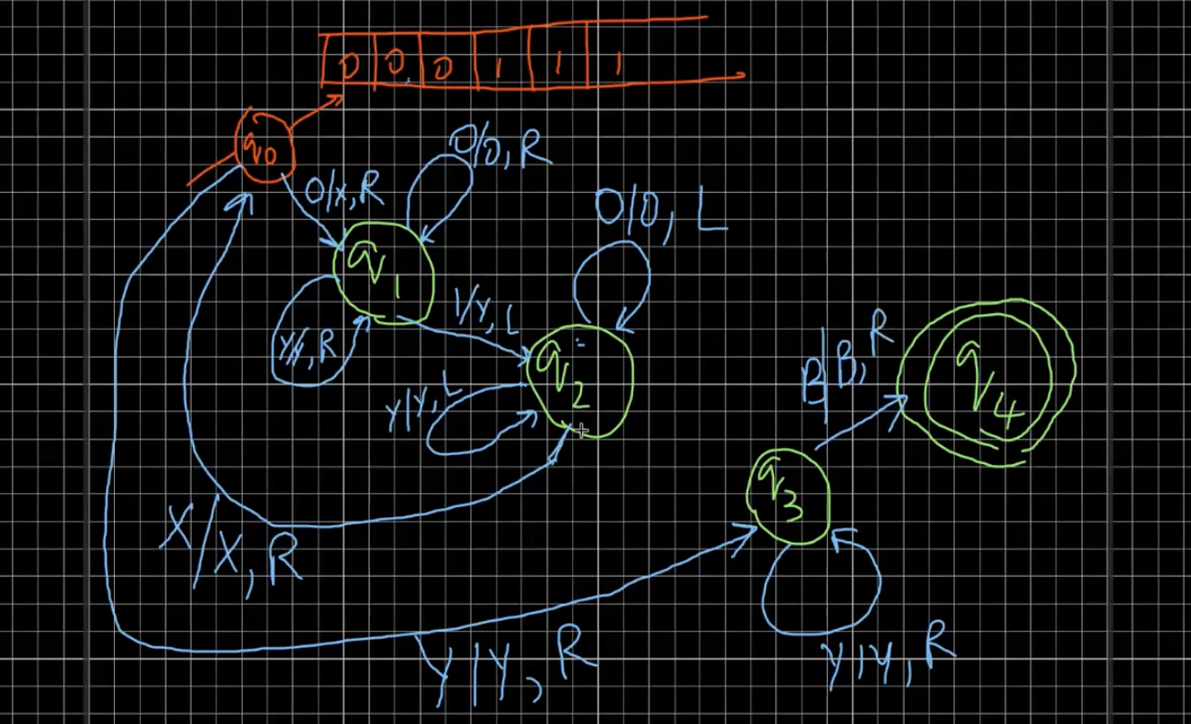
TODO Draw the above diagram again.
In a Turing machine, we halt when there is no move possible.
Formally, a Turing machine is defined as \(T = (Q, \Sigma, T, \delta, q_0, B, F)\) where \(\delta: Q \times T \to Q \times T \times \{L, R\}\). There are many variations possible to this machine which we shall show are equivalent to this simple definition. For example, we can have multiple tapes, output tape, non-determinism, etc.
Is countable same as enumerable? Countable implies that there is a one-to-one mapping from the elements in the set to natural numbers. This definition is equivalent to that of enumerability.
A Turing machine can enumerate a language. A language is recursively enumerable if a Turing machine can enumerate it.
\(\Sigma^*\) is enumerable but there are languages in \(\Sigma^*\) which are not enumerable.
The theory of Turing machines was developed in the 1930s.
Consider the derivation \((q_0, w_{inp}) \vdash^*_M (q_k, x)\) where the machine halts. A machine halts when there is no move at any given state. If \(q_k \in F\) and the machine \(M\) halts, then \(M\) accepts \(w_{inp}\).
Variations of Turing Machines
- 2-way infinite tapes
- Multi-tape heads
- Non-determinism
- Output type (write only, immutable)
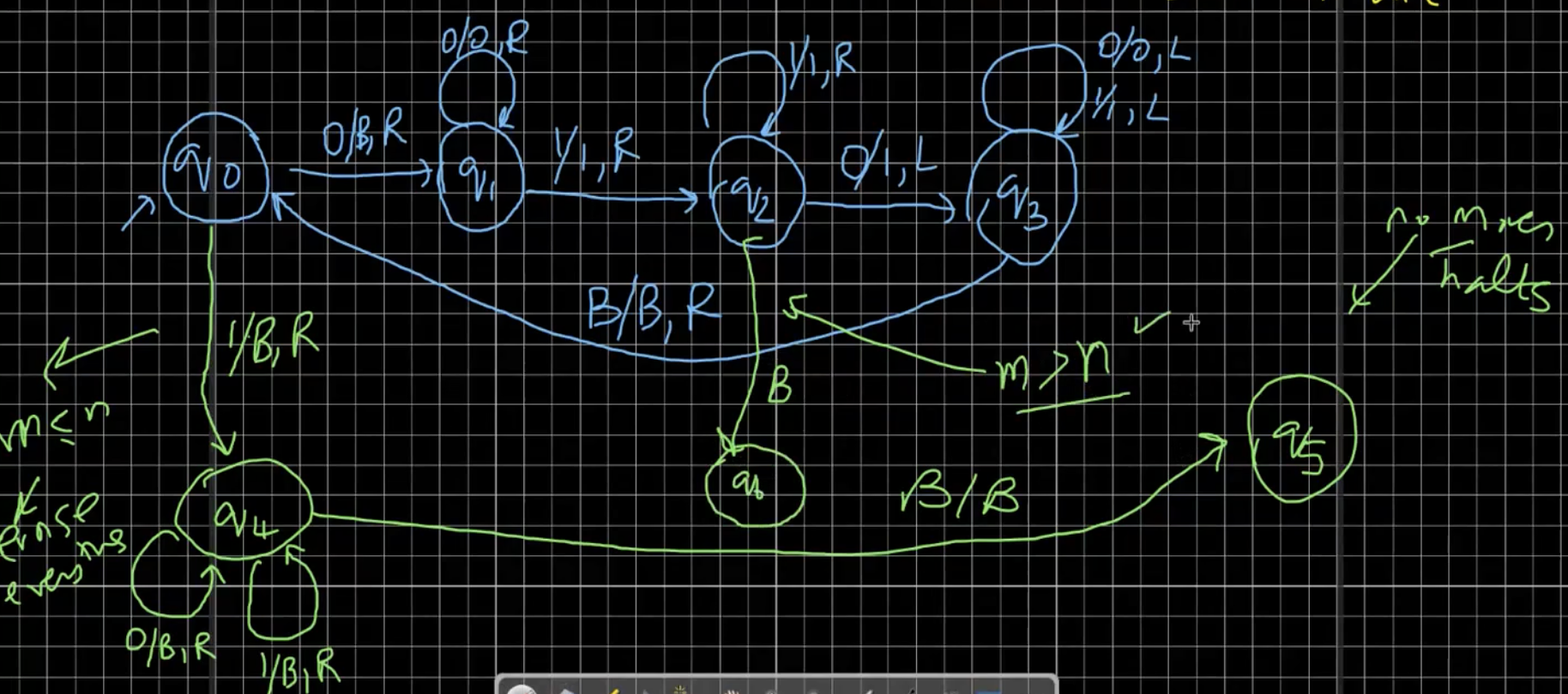
Let us try and build the Turing machine for \(L = \{a^nb^nc^n \mid n \geq 1\}\). We’ll use the following logic. In each pass, we will change 1 a, 1 b and 1 c to X, Y and Z respectively. If we have any extra a’s, b’s or c’s, then we will halt.
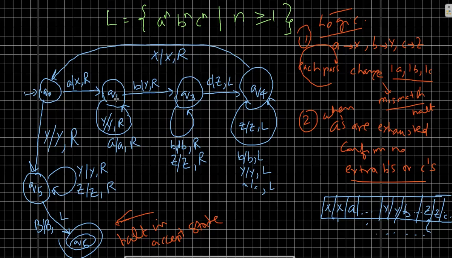
The machine is given in the above diagram.
Homework. Draw a Turing machine for the language \(L = \{ww \mid w \in (a + b)^+\}\). Hint - Think of subroutines. That is, tackle smaller problems like “Find the middle of the string”, and then match left and right.
Homework. Try \(L = \{a^n \mid n \text{ is prime}\}\)
Type-0 Grammars
These are also known as Unrestricted grammars. These are essentially same as CFGs but the LHS of rules can be any string. Consider the language \(L = \{a^nb^nc^n\mid n \geq 0\}\). The grammar can be as follows
\[\begin{align} S &\to ABCS \mid T_c \\ CA &\to AC \\ BA &\to AB \\ CB &\to BC \\ CT_c &\to T_cc \\ BT_b &\to T_bb \\ AT_a &\to T_aa \\ T_c &\to T_b \\ T_b &\to T_a \\ T_a &\to \epsilon \end{align}\]If one notices closely, then there are a few issues with this grammar. However, it is correct considering non-determinism. That is, a terminal string derived from this grammar will be in \(L\).
Homework. Write the Type-0 grammar for \(L = \{ww \mid w \in (a + b)^+\}\)
Let us go back to the \(L = \{a^nb^nc^n\}\) language. How do we come up with a deterministic grammar? We use the idea of markers.
-
1-end marker
\[\begin{align} S &\to S_1$ \\ S_1 &\to ABC \mid ABCS_1 \\ CA &\to AC \\ CB &\to BC \\ BA &\to AB \\ C$ &\to c ,\; Cc \to cc \\ Bc &\to bc ,\; Bc \to bb \\ Ab &\to ab ,\; Aa \to aa \\ \end{align}\]The problem with the above grammar is obvious. This issue is often prevented using priority rules in hierarchical grammars. Another fix for this is, adding the following set of rules
\[\begin{align} Ca &\to aC ,\; ca \to ac\\ Cb &\to bC ,\; cb \to bc\\ Ba &\to aB ,\; ba \to ab \end{align}\]Check if this is correct
-
2-end marker
TM as a recogniser
Are the set of moves on a TM a decision procedure? A decision procedure refers to a procedure that outputs yes or no for a given input. It involves correctness and termination. No, TM does not do that. For example, consider never halting TMs. Therefore, TM is a semi-decision procedure. In order to classify TM as a decision procedure, we need to show that it halts on every input. Also, we need to show that it gives the correct answer.
TM as a “computer”
Can TM replicate any function of the form \(y = f(X_1, \dots, X_n)\) where the arguments belong to $\mathbb N$. Yes, it can be done. What should a Turing machine do when we give invalid arguments to partial functions? It should never halt. On total functions, the TM must always halt and give the correct answer. For example, we have the following TM for \(f(x, y) = max(0, x - y)\). Numbers \(x\) and \(y\) are written consecutively on the tape in unary form separated by a \(1\).
If the TM has to halt when \(w \not \in L\), then we shall see that this set of TMs will only recognise recursively enumerable languages. For TMs to accept all the enumerable languages, we must allow the TM to not halt for certain inputs.
TM as an enumerator
Such TMs do not take any input. It continuously writes input on the tape and never halts. The TM prints a sequence that looks like the following \(w_1 \# w_2 \# \dots\) for each \(w_i \in L\). The machine halts if \(L\) is finite, but doesn’t otherwise. \(L\) is recursively enumerable iff a TM can enumerate the language.
Semi-Decision Procedure - Given \(M_1\) for \(L\) as an enumerator, construct \(M_2\) as a recogniser for \(L\). In \(M_2\), we can just check if the given input is present in the list of words printed by \(M_1\). Now, we have come up with a semi-decision procedure based on an enumerator.
Our goal is to determine if there are any functions that cannot be computed by TMs. Or rather, are there any languages that TM cannot enumerate or recognise. Enumeration and Recognition are equivalent (hint: dovetailing).
Recursive Function Theory
Let \(N = \{0, 1, \dots\}\). Any function we consider will be of the form \(f: N^k \to N\). How do we define these functions? We start with base cases and recursion. To define these functions, we shall define some basic functions that will be used to define the others.
- Constant function - \(C^k_n(x_1, \dots, x_k) = n\) for all \(x_1, \dots, x_k \in N\).
- Successor functions - \(S(x) = x + 1\).
- Projection function - \(P^k_i(x_1, \dots, x_i, \dots, x_k) = x_i\) for \(1 \leq i \leq k\).
We move on to more primitive recursive functions.
- Composition - \(f(x_1, \dots, x_k) = h(g_1(x_1, \dots, x_k), \dots, g_m(x_1, \dots, x_k))\)
Primitive recursion is given by
- Basecase - \(f(0, x_1, \dots, x_k) = g(x_1, \dots, x_k)\)
- Recursion - \(f(S(y), x_1, \dots) = h(y, f(y, x_1, \dots, x_k), x_1, \dots, x_k)\)
For example, the formal definition of \(+\) is given by
\[\begin{align} +(0, x) &= P^1_1(x) \\ +(S(y), x) &=h(y, +(y, x), x) \\ h(y, +(y, x), x) &= S(+(y, x)) \end{align}\]There are functions which are not primitive recursive.
We shall see that primitive recursion is not expressive enough, Adding “minimization” to our set of rules will help us define any total function. We shall also see Equational Programming that is Turing-complete.
As we have seen earlier, we are using 3 base functions - constant, successor, and projection. Composition is depicted as \(f = h \circ (g_1, \dots, g_m)\).
Primitive-Recursion in layman’s terms refers to recursion using for loops. We write the functions as \(f = \rho(g, h)\) where \(g, h\) are the same functions that are used in the recursive definition. For example, \(add \triangleq \rho(P_1^1, S \circ P_2^3)\). The recursion must be of this form. The formal definition of \(mult\) is given by \(mult \triangleq \rho(C_0^1, add \circ (P_1^3, P_2^3))\).
How do we write functions such as \(div\). Do we need if-then-else notion in our theory? Before we define this, let us try to define \(prev\) functions. We will define that \(prev(0) = 0\) for totality of the function. Then, we can define the function as \(prev \triangleq \rho(C_0^0, P_1^2)\). Using, \(prev\) we can define \(monus\) as \(monus(y, x) = x \dot- y \triangleq \rho(P_1^1, prev \circ P_2^3)\).
Now, to introduce the notion of booleans, we define \(isZero \triangleq \rho(C_1^0, C_0^2)\). We can use this function to utilise booleans. Similarly, \(leq \triangleq \rho(C_1^1, isZero \circ monus \circ (S \circ P_1^3, P_3^3))\). Using similar logic, we can implement looping and branching.
We will now see the limitations of primitive-recursion.
Limitations of primitive recursion
We have seen composition as \(h \circ (g_1, \dots, d_n)\). This concept is equivalent to passing parameters to functions in programming. To refresh the shorthand notion of primitive recursive functions, we define if-then-else as \(if\_then\_else(x, y, z)\) as \(y\) when \(x > 0\) and \(z\) otherwise. Therefore, \(if\_then\_else(x, y, z) = \rho(P_2^2, P_3^4)\). Using this, we define
\[\begin{align} quotient(x, y) &\triangleq \rho ( ite \circ (P_1^1, 0, \infty), \\ & ite \circ (P_3^3, ite \circ ( \\ &monus \circ (mult \circ (P_3^3, S\circ P_2^3) , \\ &S \circ P_1^3) , P_2^3 , S \circ P_2^3), \infty) ) \end{align}\]Ackermann function
Many mathematicians tried to show that primitive recursion is not enough to represent all functions. In this pursuit, Ackermann came up with the following function
\[\begin{align} A(0, x) &= x + 1\\ A(y + 1, 0) &= A(y, 1) \\ A(y + 1, x + 1) &= A(y, A(y + 1, x)) \\ \end{align}\]Similarly, there is a ‘91-function’ that Mc Carthy came up with. It is given as
\[M_c (x) \begin{cases} x - 10 & x> 100 \\ M_c(M_c(x + 11)) & \text{otherwise} \end{cases}\]The above function always returns \(91\) for \(x < 100\). However, it requires a lot of recursive calls for evaluating its value.
All primitive functions are total
The converse of the above statement is false. For example, the Ackermann function is not primitive. The idea is to show that any \(f\) defined using primitive recursion grows slower than \(A(n_f, y)\) for some \(n_f\). Using Godel numbering we can count all the possible primitive recursive functions.
Partial Recursive functions
We use the idea of minimisation to define partial functions and also increase the expressive power of our definitions. We have the following definition
\[\mu(f)(x_1, \dots, x_k) \triangleq \begin{cases} z & \forall z_1 < z \; f(z_1, x_1, \dots, x_k) > 0 \land f(z, x_1, \dots, z_k) = 0\\ \end{cases}\]Notice that the first case in the above definition behaves like a while loop, as it gives the smallest value of \(z\) that renders the function zero. The ‘partiality’ in the function definition comes from the fact that \(f\) may never be zero.
The Church-Turing thesis states that all definable functions that can be defined using primitive recursion, minimisation, and substitution can be computed by a Turing machine. There is no proof for this yet. The set of these functions is the set of ‘all effectively computable functions’. However, there are undecidable functions that are not computable by a TM.
Equational Logic
This paradigm has the same expressive power as primitive recursion but is easier to express. To start off, we consider the function \(leq\). We will define \(N\) as \(\{0, S(0), S(S(0)), \dots\}\). We write the rules as
\[\begin{align} leq(0, x) &= S(0) \\ leq(S(x), 0) &= 0 \\ leq(S(x), S(y)) &= leq(x, y) \end{align}\]This way of writing rules is known as Pattern matching. Similarly, \(gcd\) is given by
\[\begin{align} gcd(0, x) &= x \\ gcd(add(x, y), x) &= gcd(y, x) \\ gcd(y, add(x, y)) &= gcd(y, x) \\ \end{align}\]In the above definition, the pattern matching is semantic and not syntactic. The syntactic pattern matching definition uses \(if\_then\_else\). However, note that \(if\_then\_else\) is always assumed to be calculated in a lazy manner. That is, the condition is evaluated first and the corresponding branch is then evaluated. If the expressions in the two branches are evaluated along with the condition, then there is a chance that the computation never ends.
Also, the factorial function \(fact\) is given by
\[\begin{align} fact(0) &= S(0) \\ fact(S(x)) &= mult(S(x), fact(x)) \end{align}\]Another way of writing the factorial function using tail recursion is
\[\begin{align} f(x) &= f_a(1, x) \\ f(y, 1) &= y \\ f_a(y, S(x)) &= f_a(y\times S(x), x) \end{align}\]Notice that the first definition of \(fact\) is very inefficient compared to the latter. The second definition does inline multiplication with the arguments carrying the answer. However, the values are pushed on to the stack in the case of the first definition. These concepts of optimisation come to great use in building compilers.
Term-rewriting
We have seen 3 computation paradigms
- Turing machine
- Type-0 grammars
- Partial recursive functions
Now, we shall see a 4th paradigm called as term rewriting.
We have terms and domains. There a few constructors involved with a domain. For example, we have \(0, S\) for \(N\). Also, for lists we have \(nl\) (empty list) and \(\bullet\) (cons/pipe). We use them as follows
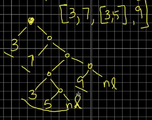
There are also constants (\(0\)) and function symbols/constructors (\(S\)). Termination is guaranteed in normal forms. We also want unique normal form. This will ensure that a term gives a single answer with different recursions (confluence). If we get two answers, we call it ill-defined systems.
To understand this better, we shall define \(exp\).
\[\begin{align} exp(x, 0) &= s(0) \\ exp(x, S(y)) &= mult(x, exp(x, y)) \end{align}\]\(max\) is defined as
\[\begin{align} max(0, y) &= y \\ max(S(x), S(y)) &= max(x, y) \\ max(x, 0) &= x \\ \end{align}\]Lists
Suppose we want to define \(app\). We then have
\[\begin{align} app(nl, y) &= y \\ app(\bullet(x, y), z) &= \bullet(x, app(y, z)) \end{align}\]Similarly,
\[\begin{align} rev(nl) &= nl \\ rev(\bullet(x, y)) &= app(rev(y), \bullet(x, nl)) \end{align}\]Homework. Show that \(len(x) = len(rev(x))\)
How do we sort a list of numbers?
\[\begin{align} sort(nl) &= nl \\ sort(\bullet(x, y)) &= ins(x, sort(y)) \\ ins(x, nl) &= \bullet(x, nl) \\ ins(x, \bullet(y, z)) &= \bullet(\min(x, y), ins(\max(x, y), z)) \end{align}\]Homework. Try quick sort and merge sort.
Termination
We have termination on \(N\) due to \(>\). How about \(N \times N\)? We use lexicographic ordering. One might think it’s not well-founded. This is because \((9, 1)\) is greater than \((5, 1000)\). However, it is well-founded for finite length tuples. In case of strings, the length need not be finite in lexicographic ordering. Therefore, the ordered list need not be finite.
Homework. Give an ordering rule for multi-sets
Predicates and Branching
It is easier to express these things in the term-rewriting paradigm. I’m skipping these for brevity.
Can we write \(isPrime\), \(gcd\), and \(nth-prime\)? This paradigm naturally develops to Functional Programming. It’s essentially writing everything in terms of functions as we’ve been doing so far.
Logic Programming
Suppose we give the black-box the input \(x + 3 = 10\). Can we determine \(x\)? Can we ask multiple answers in case of \(u + v = 10\)? It is possible to do so in logic programming. We do this by passing parameters by unification. That is, we try to convert the parameters \(u, v\) to look like the parameters given in the rules of \(+\). This is known as backtracking.
Term matching is don’t care non-determinism. There might be multiple possible reductions at any given situation, and all will lead to the same answer in case of well-formed normal forms. Also, all the paths should terminate.
What are the strategies for computing normal forms?
- Hybrid - Check if sub-term matches rule-by-rule
- Innermost - Many programming languages adopt this. Evaluate the “lowest” redex first.
- Outermost - This is lazy evaluation. We evaluate topmost redex first.
Redex is a sub-term where a rule can be applied.
And then, sir lost his connection :D
Aside. Write primality test function using primitive recursion. \(\begin{align} prime(0) &= 0 \\ prime(S(x)) &= g(x, S(x)) \\ \\ g(0, y) &= 0 \\ g(S(x), y) &= ite(isZero(y), 1,\\ &ite(isZero(monus(S(x), gcd(S(x), y))), 0, g(x, y))) \\ \\ gcd(0, y) &= y \\ gcd(S(x), y) &= ite(gte(S(x), y), \\ &gcd(monus(S(x), y), y), gcd(y, x)) \end{align}\)
We were discussing the definition of \(quotient\) in the previous lecture. In terms of minimisation, we can write the definition as
\[\begin{align} quotient(x, y) &= \mu(f)(x, y) \\ f(k, x, y) &= y*k > x \end{align}\]Encoding Turing machines
Let us consider the example of enumerating all the finite subsets of \(N\). A subset \((n_1, n_2, \dots, n_k)\) is represented as \(m = p_1^{n_1} \times \dots \times p_k^{n_k}\) where \(p_1, \dots, p_k\) are the first \(k\) prime numbers. Note that we need to ignore trailing zeros for this.
Can we enumerate Turing Machines? Let us try to encode a Turing Machine as a bit string. The core idea is that a Turing Machine has a finite set of states. We can encode a transition in the following way - Suppose we have the transition \(\delta(q_3, X_1) = (q_7, X_2, D_0)\). Then, the bit string corresponding to this is \(11\; 000 \;1 \; 0000000 \; 1\; 0 \; 1 \; 00 \; 1 \; 0 \; 11\) Here, a \(1\) just acts as a separator, and every state, tape symbol and direction are encoded in unary format. A substring \(11\) represents the start of a transition, followed by \(q_3, q_7, X_1, X_2, D_0\) for the above example. This way, we can list all the transitions of the Turing Machine. All the transitions can be enclosed between a pair of substrings \((111, 111)\). Now, we just need to add the set of final states.
Instead of listing out all the final states, we can convert the Turing Machine to an equivalent TM which has a single finite state.
Homework. Prove that the above conversion can be done for any Turing Machine.
Now that we have encoded a TM, how do we enumerate the set of all TMs? We know how to enumerate bit strings based on the value and the length (ignore leading \(0\)‘s for non-ambiguity). We need out to weed out the bit strings that do not represent a valid TM.
What features are present in a bit string that represents a TM? It needs to start with \(111\), and end with \(111\). If there is a \(11\) in between the above substrings, there need to be at least 4 \(1\)‘s in between with appropriate number of \(0\)’s in between. This concludes our discussion on encoding TMs.
Variants of TM
Let us consider the time of execution with a single computer and \(n\) computers. Any task will have at most \(n\) times speedup when done on \(n\)-computers in comparison to a single computer (generally). For example, matrix multiplication can be heavily parallelised. However, tasks such as gcd calculation of \(k\) numbers is inherently sequential and it is not easy to speed it up using parallel computation.
Now, we shall consider variants of TMs and show equivalence of each with the 1-way infinite tape variant.
2-way infinite tape
It is easy to see that a 2-way infinite tape can be restricted of the left movement beyond a point to simulate all the 1-way infinite tape machines.
To prove the other direction, we will consider a multi-track 1-way TM. That is, every cell will now contain 2 elements. The basic idea is that a 2-way machine of the form \(\dots \mid B_1 \mid B_0 \mid A_0 \mid A_1 \mid \dots\) will be converted to \((A_0, C) \mid (A_1, B_0) \mid \dots\).
The states in the 2-way machine will be separated based on whether the transition is on the left side of the tape or the right side. Then, based on the side, we will work on the first element in the tuple of each cell or the second element. The formal proof is left to the reader.
Multi tapes
There are multiple tapes under a single control. Therefore, each transition is represented as \(( X_1, \dots, X_k )\mid ( Y_1, \dots, Y_k) , (D_1, \dots, D_k)\). One can see that all the logic boils down to the Satan-Cantor puzzle.
Again, one direction of the equivalence is straightforward. The other half involves converting a \(k\)-tuple to a natural number.
Non-Determinism
The equivalence can be shown in a similar way as that of regular languages.
k-head machine
We have a single tape which has multiple heads that move independently.
Offline TM
The input tape never changes. That is, the actions are read-only.
Universal Turing Machine
The intention is to build a general purpose computer. Recollect that a Turing Machine is represented as \(M = (Q, \Sigma, T, \delta, q, B, F)\).
Every Turing Machine has an equivalent TM
- whose alphabet is \(\{0, 1\}\) and the set of tape symbols is \(\{0, 1, B\}\), and
- has a single final state.
\(L\) is
- recursively enumerable - there exists a TM (recogniser) that accepts \(L\) (need not halt on wrong input, think of recogniser built from enumerators).
- recursive - there is a TM that accepts \(L\) which halts on all inputs.
For example, consider the language that accepts a pair of CFGs \((G_1, G_2)\) if \(L(G_1) \cap L(G_2) \neq \phi\). To show that this language is recursively enumerable, we will give a high level algorithm in terms of primitive steps that we know can be converted to a TM. We consider the following algorithm.
- Enumerate L(G_1) // enumerate w, check G_1 =>* w (CYK)
- For each w in L(G_1) check if G_2 =>* w
Now, if we generate a word and check for the word in the other grammar alternately, then the algorithm will halt if the input is acceptable. However, it is not guaranteed to halt in case of unacceptable input for this algorithm. Does that mean the language is recursively enumerable?
We need to show that we can’t construct an algorithm that halts in case of an unacceptable input. Then, we can conclusively state that the language is recursively enumerable.
In conclusion, there are language that are recursively enumerable, and languages that are not recursively enumerable. The set of recursive languages are a strict subset of the set of recursively enumerable languages.
Non-recursive language
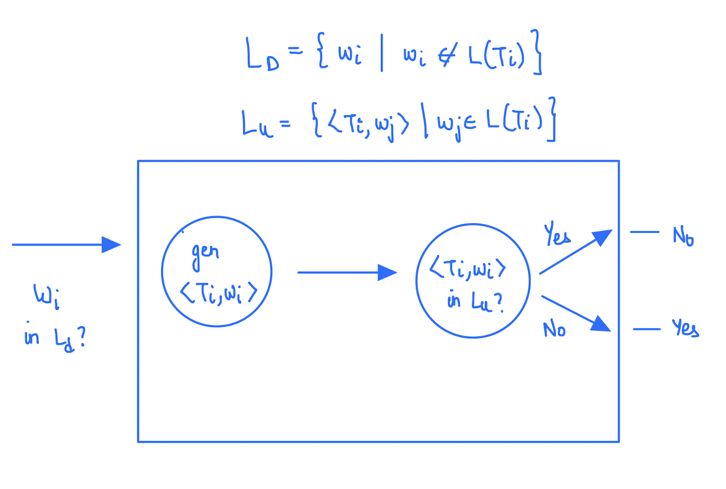
We know that we can enumerate all TMs and all \(w \in \Sigma^*\). Then, we draw a 2D infinite bit matrix A where \(A_{ij}\) tells whether \(w_i \in M_j\). Now, we use the Cantor’s diagonalization argument to conclude that \(L_d = \{i \mid A_{ii} = 0\}\) is not recursively enumerable. Genius proof based off Barber’s paradox.
If \(L\) is not recursively enumerable, then \(\bar L\) is also not recursively enumerable. That is, show that if TM accepts \(L\), then it must also accept \(\bar L\).
One might ponder on how we construct the table \(A\) when some TM may not halt for a few inputs. The important distinction is that, we are “defining” this table conceptually and not “computing” it. The concept of dovetailing also comes to use here.
Recursively enumerable but not Recursive
The language of the Universal Turing Machine is the required example. We formally define this language as \(L_u = \{( M, w) \mid\ M \text{ halts on } w\}\).
Equivalently, we are trying to write a Python script that takes another Python script as input along with some arguments. This script should halt when the input python script halts on the input argument, and need not halt otherwise. Basically, we are trying to build a simulator TM.
No lectures 32 and 33.
Undecidability
A language \(L \subseteq \Sigma^*\) is recursive if there is a Turing Machine \(M\) that halts in an accept state if \(w \in L\) and in a reject state if \(w \not\in L\). It need not halt in reject states for recursively enumerable languages. The algorithms similar to the latter TMs are semi-decidable.
We were looking for languages that are not recursively enumerable \(L_d\) and languages that are recursively enumerable but not recursive \(L_u\). For the latter set, we had seen the universal TM. We also have the language of “polynomials that have integer roots”. How do we show that this is recursively enumerable? The key idea lies in encoding polynomials as a number. The motivation for this language comes from Hilbert’s 10th Problem.
Another example for an undecidable problem is the Halting Problem.
Let us continue the discussion on \(L_u\) and \(L_d\) from the last lecture. We had constructed a matrix \(A\) and showed using the diagonalization argument that there are languages that are not recursively enumerable. However, we did not address two issues
- There are multiple TMs that accept the same language - It does not matter.
- How do we fill the table? - Computation vs Definition.
Also, all the languages defined by each row \(A_i\) in the matrix form the set of recursively enumerable languages.
We had defined \(L_u\) as \(\{(M_i, w_j) \mid M_i \text{ accepts } w_j \}\). We will show that this language is recursively enumerable by constructing a Turing Machine \(M\) that accepts this language. The input tape will initially have the encoding of \(M_i\) followed by the encoding of \(w_j\). Now, we use two more tapes
- One for copying \(w_j\)
- Another tape for keeping track of the state in \(M\), starting with state 0.
Now, we give the higher level logic of \(M\).
- Validate \(M_i\). This can be done using a TM.
- Run \(M_i\) step-by-step. Pick the top state from the 3rd tape, find the corresponding move from the first tape, and update the 2nd and 3rd tapes.
The last two tapes help simulate any input TM. In conclusion, we have constructed a universal TM. Therefore, the TM paradigm is powerful enough to perform self-introspection.
Note that we have still not shown \(L_u\) is not recursive. We will use the properly of \(L_d\) not being recursively enumerable to show this.
Let us continue the discussion on the Universal Turing Machine. The encoding of a move \(\delta(q_i, X_j) = (q_k, Xl, D_m)\) in a Turing Machine is \(0^i10^j10^k10^l10^m\). The universal TM works in 3 steps
- Decode/Validate
- Set up the tapes
- Simulate
Also, we had shown that \(L_u\) is recursively enumerable by the construction of the universal TM. Suppose, there is a TM that halts every time for \(L_u\). Now, we will show that \(L_u\) is recursive then \(L_d\) is recursive. To do that, we will convert \(L_d\) into an instance of \(L_u\).
Here, we can see that we are able to answer the question \(w_i \in L_d\) by constructing a TM using the Universal TM. That is, if the Universal TM is recursive, then \(L_d\) is also recursive. Think.
Reduction Technique
To understand this technique, consider the following two problems
- \(L_{ne} = \{( M ) \mid L(M) \neq \phi\}\) - Machine accepts at least one string
- \(L_{rec} = \{( M ) \mid L(M) \text { is recursive}\}\) - Machine halts on all inputs
We can show that both are recursively enumerable. The first language can be shown as recursively enumerable using dovetailing (words and moves being the dimensions). To show non-recursivity, we convert \(L_d\) or \(L_u\) to an instance of this language. We need to try and come up with an algorithm that halts for machines with empty languages.
How do we do this?
The second problem is a little bit more difficult.
In conclusion, given a language
- To prove that it is recursive, we need to construct a TM that halts on all inputs.
- To prove that it is recursively enumerable, we just need to construct a TM that halts on good inputs. To show that it is not recursive, we need to use reductions probably.
- To prove non recursively enumerable, we need to show that we can’t construct any TM.
TM is a powerful model as it is universal (self-referential), and it has many undecidable problems. They can represent Type-0 Grammar, Partial Recursive functions, and RAM (random access mechanism).
Post Correspondence Problem
Post is a mathematician. Consider the following table
| w | x |
|---|---|
| 1 | 111 |
| 1011 | 10 |
| 10 | 0 |
Now, take the string \(101111110\). Can we decompose this string in terms of \(w_i\) or \(x_i\)? For example, we can decompose the string as \(2113\) in terms of \(w's\) and \(2113\) again in terms of \(x’s\). These decompositions need not be unique.
So, PCP is stated as follows.
Given \(w = \{w_i \mid w_i \in \Sigma^* \}, x = \{x_i \mid x_i \in \Sigma^*\}\) and a string \(s \in \Sigma^*\), we need to be able to come up with decompositions \(s = w_{i1} \dots w_{il}\) and \(s = x_{j1}\dots x_{jl}\) such that \(ik = jk\) for \(k \in \{1, \dots, l\}\).
Consider the following table.
| w | x |
|---|---|
| 10 | 101 |
| 011 | 11 |
| 101 | 011 |
Now, for any string \(s\), we will not be able to come up with decompositions that are equal for the above sets.
The reason we came up with this problem, is to show that PCP is undecidable (not recursive). That is, no TM can halt correctly on all PCP instances. However, it is recursively enumerable as we can enumerate all sequences fairly. This can be shown by a reduction of \(L_u\) to PCP.
Let us now consider another problem - Ambiguity of CFGs. Can we build a TM that halts with a ‘yes’ if the input CFG has an ambiguity and with a ‘no’ is it does not. In an ambiguous grammar, a single word has multiple derivations in the grammar. That is, we have multiple structurally different derivation trees. Using this problem we are trying to show the importance of direction of reduction. We know that PCP is undecidable. Therefore, we need to reduce PCP to an instance of the CFG problem. That is, we’ll essentially show that is the CFG problem is decidable, then so is PCP.
PCP is essentially a pair of sets of strings. What is the grammar corresponding to these sets such that when PCP has a solution, the grammar is ambiguous and unambiguous otherwise? We introduce \(k\) new symbols \(a_1, \dots, a_k\). We construct the following grammar
S -> Sa | Sb
Sa -> w_i Sa a_i | w_i a_i
Sb -> x_i Sb a_i | x_i a_i
It is easy to see that this grammar meets our requirements. To prove this, we need to show the proof in two directions
- If PCP has a solution, then G is ambiguous
- If G is ambiguous, then PCP has a solution. Here, we need to show that ambiguity happens only due to
SaandSb.
Why did we introduce
a?
Note. To show problem A is undecidable knowing that problem B is undecidable, we essentially show that A is a subroutine of B.
Properties of Recursive Languages
If \(L_1\) and \(L_2\) are both recursive, then so are
- \[L_1 \cup L_2\]
- \[L_1 \cap L_2\]
- \[L_1 - L_2\]
- \[L_1^c\]
- \[L_1L_2\]
The intersection and complement closure break in case of recursively enumerable languages (?)
Note. Don’t get confused into thinking there are three (disjoint) kinds of sets: decidable, semi-decidable, and undecidable. There are two kinds: decidable and undecidable. Semi-decidable falls under undecidable.
NP-Completeness
Decision Problems
These are a class of problems that deal with problem instances like Fermat’s last theorem - \(\forall n > 2\exists a, b, c, a^n + b^n = c^n\)? We also have the law of excluded middle in decision problems - The answer is either ‘yes’ or ‘no’.
Optimisation problems can be converted to a decision problem.
Decidable Problems
We solve these problems by building a brute-force TM - generate and test method. For example, consider the problem of finding a vertex cover in a graph of size \(k\). Now, the TM will enumerate all subsets of size \(k\) and check each one for vertex cover conditions.
We come up with “algorithms” for these problems and check their efficiency. Apart from time and space complexity, we also consider descriptive (Kolmogorov) complexity. It refers to the program size. In our case, it refers to the size of the TM.
Complexity Classes
Given two problems, which problem is “more difficult”? The difficulty criterion we consider is time. We define two classes of problems \(P\) and \(NP\).
- P is the class of (decision) problems that can be solved in “polynomial time” by a deterministic Turing Machine \(M\).
- PSPACE refers to the class of problems that use polynomial number of cells in the tape.
- NP is the class of (decision) problems that can be solved in polynomial time by non-deterministic TM. This is equivalent to guessing a solution in polynomial time followed by checking using a deterministic TM in polynomial time. The claim is that this is same as a non-deterministic TM. We shall use this technique to show that problems are in NP. That is, we’ll show that we can guess in P-time and verify in P-time.
For example, let us try to show vertex cover problem is in \(NP\). Aside - A polynomial algorithm was developed in the 1980s for the problem “Is \(n\) a prime number” in IITK (Manindra Agarwal).
More difficult problem
Given \(L_1\) and \(L_2\), which one is more difficult? We use reduction to answer this question.
\[L_1 \leq_{P} L_2\]If \(L_1\) can be converted to an instance of \(L_2\) in polynomial time, then we have the above defined relation. That is, \(L_2\) is at least as difficult as \(L_1\).
Completeness
We try to determine the most difficult problem amongst all the problems. To start off, we define that \(L_{sat}\) belongs to NP-complete set. This problem refers to the satisfiability of propositional logic expressions.
Every problem in \(NP\) can be reduced to \(L_{sat}\). In some sense, \(L_{sat}\) is the most difficult problem. But how did we come to this conclusion without knowing all the problems in \(NP\)? We can show that any non-deterministic TM can be reduced to \(L_{sat}\).
We define hard problems as anything not in \(P\). There are problems that are more difficult than the ones in \(NP\)!
We classify decidable problems as the set of recursive languages. These problems can be further classified as
- Deterministic TM takes only polynomial number of steps in terms of the input size to halt.
-
A non-deterministic TM takes polynomial number of steps.
- A non-deterministic TM needs \(\Omega (2^n)\) number of steps.
SAT Problem \(P_{sat}\)
Given a well formed formula \(F\), is \(F\) satisfiable? A well formed formula is a formula that is formed via the base case (propositional variables) and inductive rules (using connectors like negation, ‘and’ and ‘or’).
This problem can be solved via brute force but that is exponential. So we now ask the following questions
- Is \(P_{sat} \in P\)?
- Is \(P_{sat} \in NP\)?
We’ll answer the second question first. It is easy to construct a non-deterministic TM that solves the problem in polynomial steps. We can generate a random guess (bit string) and verify (check satisfiability) in polynomial steps. This procedure is the way to show that any problem is in \(NP\).
Comparison of Problems
Let us revisit the topic of \(\leq_{P}\). \(P_{sat} \leq_{P} 3\text{-}SAT\), and \(3\text{-}SAT \leq_P VC\) where \(VC\) is the vertex cover problem.
To do perform the latter reduction, we construct nodes for \(p\) and \(\neg p\) for each propositional variable in the clause. Then, we construct cliques out of each disjunction in the CNF. Finally, we connect each \(p\) with \(\neg p\). Now, if we can find a vertex cover of this graph with size \(2k\), we get the satisfiability of the 3-CNF clause with \(k\) disjunctive clauses.
- If \(F\) has a satisfying assignment, take out exactly one literal with value \(1\) out of each disjunctive clause and construct a VC out of the remaining literals. It can be shown that the vertex cover will have size \(2k\).
- If there is a vertex cover, then we can drop at most 1 node from each disjunctive clause. Also, as the size if \(2k\) we can drop exactly 1 node from each clause. Assign these dropped nodes with a value of \(1\). Now, since we have a true value in each clause, the assignment satisfies the expression.
NP-Completeness
As we mentioned before, we consider \(P_{sat}\) or \(3\text{-}SAT\) as the hardest problem. That is, for every \(Q \in NP\), \(Np \leq_P P_{sat}\).
We show this by reducing non-deterministic Turing Machines to \(P_{sat}\). To prove that a problem is NP-complete, we show
- That the problem lies in \(NP\). This step is very important as there are problems that are more difficult than \(NP\).
- Convert the 3-SAT problem (or any other known NP-complete problem) to an instance of the given problem.
We list out some problems in NP-complete set.
- 3-SAT
- Vertex Cover
- Clique in a graph
- \(k\)-coloring
- Min-cut and Max-flow
- Travelling Salesman Problem
- Hamiltonian Cycle in a graph
- Partitioning of a set of numbers such that the partitions have the same sum
- Knapsack problem
The good news about \(NP\)-complete problems is that there are many heuristics and approximations such as LAs Vegas and Monte Carlo that work well for most of the above problems.
END OF COURSE
Enjoy Reading This Article?
Here are some more articles you might like to read next: