Data Systems for Machine Learning
Introduction
Machine Learning systems have played a pivotal role in the rapid adaptation of Ai in the world today. This domain is essential for solving future problems and also making the current architectures more efficient. This is crucial considering that companies are reactivating nuclear power plants to power AI in the real-world.
Along with the progress in AI from small neural networks to large language models, there has been a development in the size of datasets as well. Big data arrived, and AI today relies on these internet-scale datasets. After all, doesn’t ChatGPT just do pattern-matching in the internet?
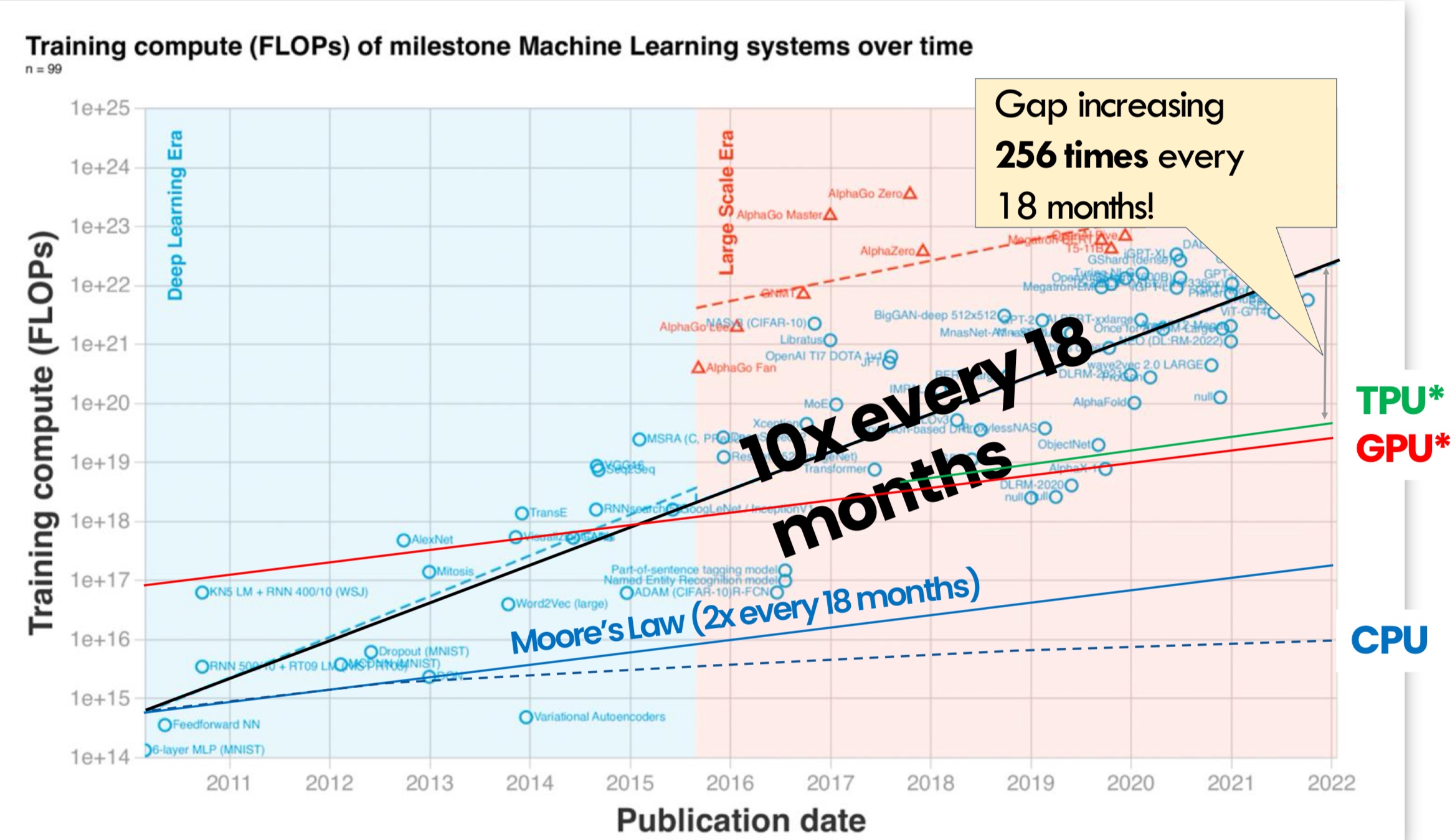
Moreover, the compute capabilities have been scaling exponentially. Just last year (2024), NVIDIA released a new super-chip architecture Blackwell that has 97 billion transistors that can reach up to 1.4 exa-flops! The largest super-computer was barely able to reach 1 exa-flop. All this power in the palm of your hand…
Richard Sutton once said, search and learning can scale unparalleled with growing computation power.
Consider the year 2012 — AlexNet made waves showing SOTA capabilities with images. They use Stochastic Gradient Descent, dropout, convolution networks and initialization techniques. Without ML systems (CUDA, etc), the code would have been 44,000 lines with days of training! With these systems (Jax, PyTorch, TensorFlow) in place, you can achieve the same result in 100 lines within hours of training.
In Practice
In industry, problems are typically of the form - improve the self-driving car’s pedestrian detection to be X-percent accurate at Y-ms latency budget. For an ML engineer is, the general approach is to design a better model with better learning efficiency followed by hyper-parameter running, pruning, distillation. An ML systems engineer would take the best model by ML researchers, specialize the implementation to target the H/W platform to reduce latency. Streamlining the entire process from development to deployment.
Overview
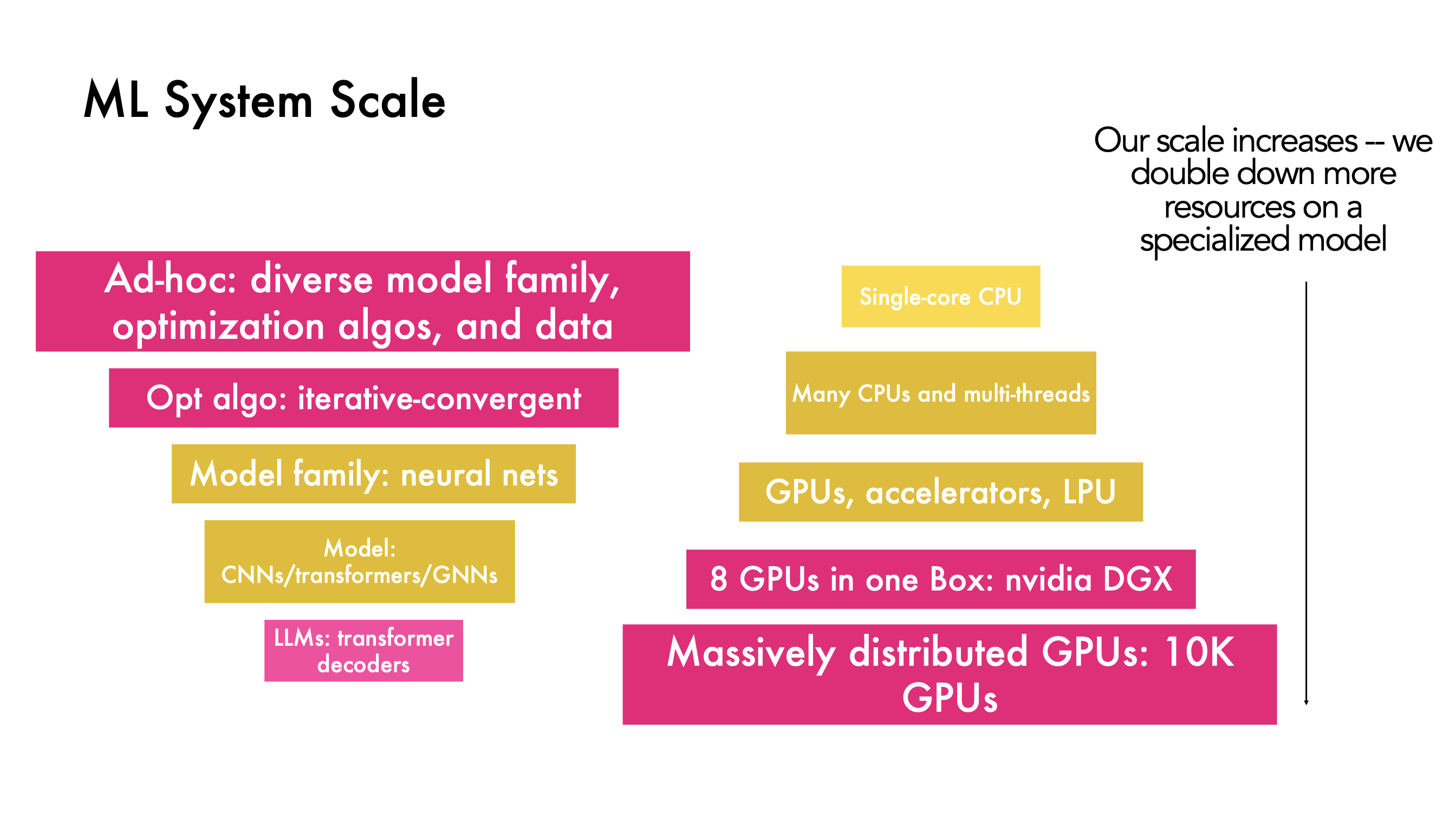
From ad-hoc methods having diverse models and optimization algorithms with various data pre-processing techniques - we have arrived at an optimal algorithm that is iterative and convergent. As our models have become more and more specialized, the computation resources scaled exponentially.
Through the course of this article, we will cover deep learning basics, computational graphs, Autodiff, ML frameworks, GPUs, CUDA and collective communication.
There are more related topics to the ones discussed here
- ML for systems
- ML Hardware design
Unfortunately, the textbook for this content is just miscellaneous research papers.
Background
DL Computation
The idea is to concatenate composable layers
\[\theta^{(t + 1)} = f(\theta^{(t)}, \nabla_L(\theta^{(t)}, D^{(t)})\]A model is a parameterized function that describes how we map inputs to predictions. The parameters are optimized using optimization methods like SGD, Newton methods, etc. A loss function guides the model to give feedback on how well the model is performing.
Having these basic definitions, we will build abstractions to map all the models being used today. It is not possible to build systems to support all models. A quick refresher of important models
- CNNs - Learnable filters to convolute across images to learn spatial features. The top 3 breakthrough architectures were - AlexNet, ResNet, U-Net. What are the important components in CNNs?
- Convolution (1D, 2D, 3D)
- Matmul
- Softmax
- Element-wise operations - ReLU, add, sub, pooling, normalization, etc.
- Recurrent Neural Networks - Many problems in nature are many-to-many. RNNs maintain an internal state that is updated as a sequence is processed. Arbitrary inputs and outputs can be generated, and any neural network can be used in the RNN architecture. The top 3 breakthrough architectures were - Bidirectional RNNs, LSTMs, GRU. What are the important components in RNNs?
- Matmul
- Element-wise non-linear - ReLU, Sigmoid, Tanh
- Underlying MLP RNNs have a problem of forgetting (\(0.9*0.9*… \approx 0\)). Additionally, they lack parallelizability - both forward and backward passes have \(O(sequence length)\).
- Transformers (Attention + MLP) - Treat representations of each element in the sequences as queries to access and incorporate information from a set of values. Transformers have an encoder part (BERT most famous) and a decoder part (GPT most famous). Along with these, DiT is one of the top 3 models. What are the important components in Transformers?
- Attention - Matmul, softmax, Normalization
- MLP
- Layernorm, GeLU, etc.
- Mixture of Experts - Voting from many experts is better than one expert. Latest LLMs are mostly MoEs - Grok, Mixtral, Deepseek-v3. A router (Matmul, softmax) is the novel component in MoE - it makes system design difficult.
Machine Learning Systems
As mentioned before, the three pillars for the systems are data, model and compute. The foal is to express as manny as models as possible using one set of programming interface by connecting math primitives.
Computational Dataflow Graph
A representation to show data flow in programs. A node represents the computation (operator) and an edge represents the data dependency (data flowing direction). A node can also represent the input/output tensor of the operator.
Example: Deep learning with TensorFlow v1
import tinyflow as tf

x = tf.placeholder(tf.float32, [None, 784]) # Forward declaration
cross_entropy = tf.reduce_mean(-tf.reduce_sum(y *tf.log(y), reduction_indices=[1])) # Loss function declaration
W_grad = tf.gradients(cross_entropy, [W])[0] # Automatic differentiation
train_step = tf.assign(W, W - learning_rate*W_grad) # SGD update rule

for i in range(1000):
        sess.run(train_step, feed_dict={x, y}) # Real-execution happens here
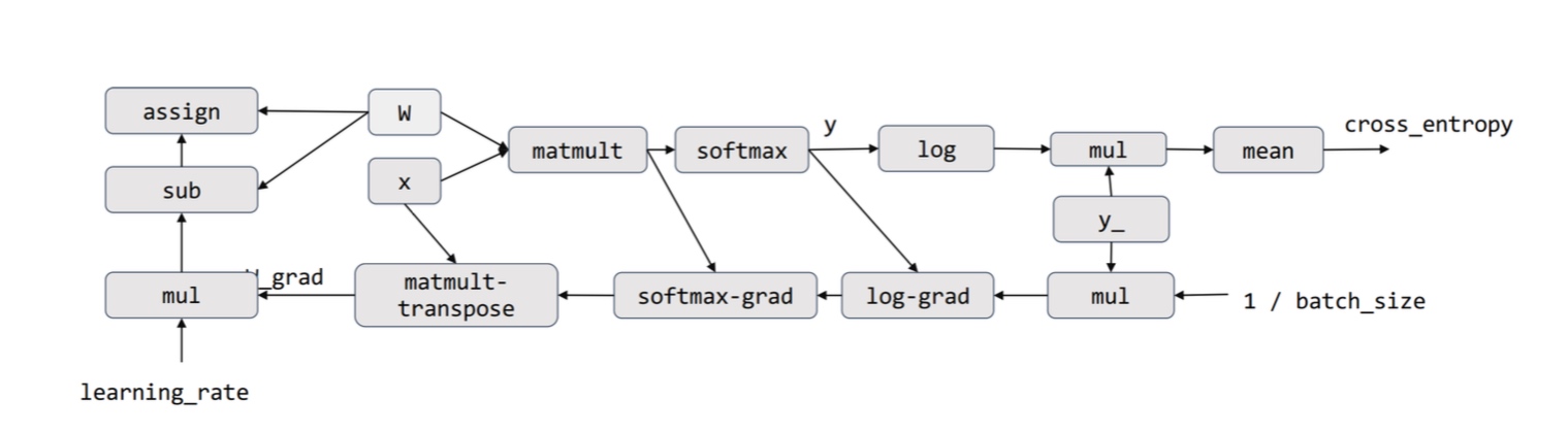
This DAG representation opens up all possibilities of optimizations. However, creating such a graph doesn’t allow flexibility - once a graph is defined, it cannot be changed based on the input.
Example: PyTorch
PyTorch also uses computational graphs, but it creates it on the fly. Previously, we had defined the graph and then executed it. Symbolic declaration vs imperative programming. Define-then-run vs Define-and-run. C++ vs Python.
What are the pros and cons?
| Good | Bad | |
|---|---|---|
| Symbolic | Easy to optimize, much more efficient (can be 10x faster) | The way of programming can be counter-intuitive, hard to debug and less flexible |
| Imperative | More flexible, easy to program and debug | Less efficient and more difficult to optimize |
How does TensorFlow work in Python then? Tensorflow has Python as the interface language.
Apart from these two famous frameworks, there were more like Caffe, DyNet, mxnet (has ability to switch between both), etc. Recently, Jax (derived from Tensorflow) has been getting more popular.
Just-in-time (JIT) compilation
Ideally, we want define-and-run during development and define-then-run during deployment. However do we combine both? PyTorch introduced a deploy mode through a decorator torch.compile(). So is there an issue with JIT? It creates only static graphs, and cannot work with conditionals or loops in the code.
Static vs Dynamic models
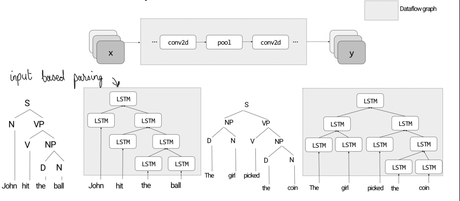 Static graphs are defined and optimized only once. The execution follows a defined computation. On the other hand, dynamic graphs depend on the input. It is difficult to express complex flow-control logic and debug. The implementation is also difficult.
As seen above, LSTMs are trying to replace the dynamics in the natural language problem.
How to handle dynamics?
- Just do Define-and-run and forget about JIT - most popular unforunately :(
- Introduce Control Flow Ops -
- Example: Switch and Merge. This can be added a computational primitive in the graph and introduce dynamics in the graph.
- These ideas are natural across all programming languages - conditionals and loops. However, the problem with this approach is that graphs becomes complex, and more importantly, how does we do back propagation? What is the gradient of “switch”? TensorFlow team has been working on this.
- Piecewise compilation and guards - This approach is better adopted than control flow.
- Case 1: A graph accepting input shapes of \([x, c1, c2]\) where \(x\) is variable. The solution is to compile for different values of \(x\) (powers of 2).
So far, we have seen representations that express the forward computations using primitives. But, how do we represent backward computations?
Autodiff (AD)
Derivative can be taken using the first order principles. However, this approach can be slow since we have to evaluate the function twice \(f(\theta + \epsilon) , f(\theta)\) and it is also error prone \(\theta(\epsilon^2)\).
To optimize the derivative calculation, we pre store the gradients of primitives and map the derivative chain rules in the computational graph. There are two ways of doing this as well
- Calculating the derivative from left (inside) to right (outside) in a network - from inputs to outputs
- Calculating it from right to left - from outputs to inputs
Both are valid approaches and we will discuss them in detail.
Forward Mode Autodiff
We start from the input nodes, and derive the gradients all the way to the output nodes. Cons - - For \(f: R^n \to R^k\), we need \(n\) forward passes to get the gradients with respect to each input. - However, it is usually the case that \(k = 1\) (loss) and \(n\) is very large.
If this is confusing, think of it this way - we want the gradient of output with respect to all parameters to update weights. However, forward mode calculates the gradient of inputs with respect to all parameters.
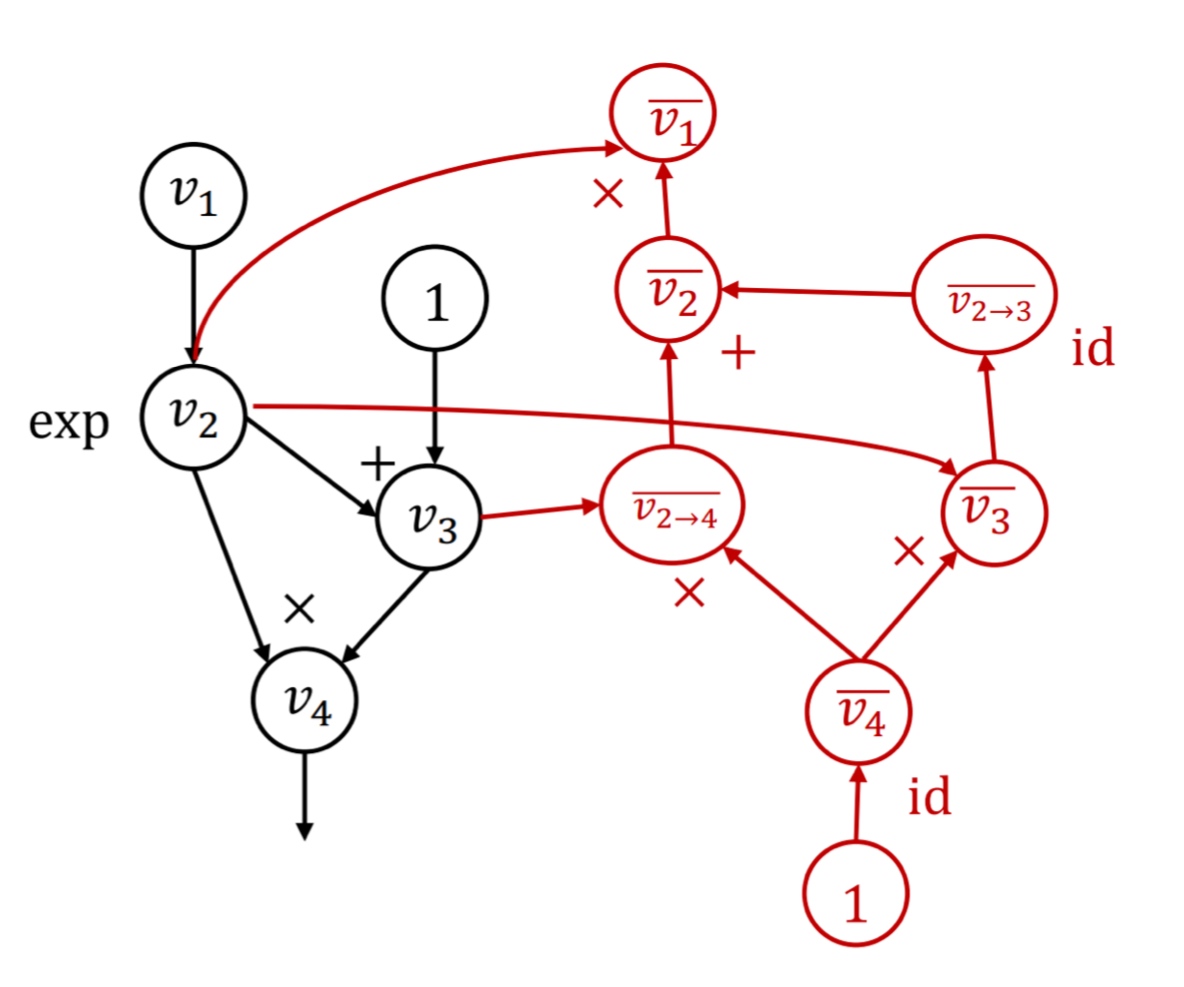
Reverse Mode Autodiff
We define the quantity adjoint \(\bar v_i = \frac{\partial y}{\partial v_i}\). We then compute each \(\bar v_i\) in the reverse topological order of the graph. This way, we can simply do one backward pass to get the necessary gradients.
In some scientific scenarios, we can have \(k >> n\) where the forward mode can be more efficient.
What are the size bounds of the backward graph as compared to the neural network?
We construct backward graphs in a symbolic way to reuse it multiple times.
Backpropagation vs. Reverse-mode AD
In old frameworks like Caffe/cuda-convnet, the backward computations were done through the forward graph itself. Newer frameworks like Tensorflow and PyTorch construct the backward graph explicitly. The reasons to do so are -
- Explicit graphs allow backward computation with any input values. They have flexibility to even calculate gradient of gradients.
- Having an explicit backward graph can help optimization!
- Gradient update rules can be efficiently implemented.
Gradient update rules
Typically done via gradient descent, the weights are updated with the gradients with the following simplified rule
\[f(\theta, \nabla_l) = \theta - \eta \nabla_L\]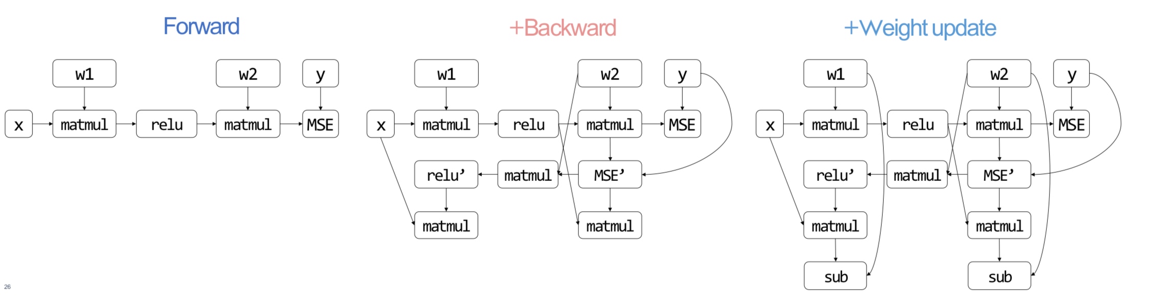
Architecture Overview of ML systems
The aim is to make the systems fast, scalable, memory-efficient, run on diverse hardware, energy efficient and easy to program/debug/deploy. Phew.
We have discussed dataflow and Autodiff graphs. However, there are numerous things that can be added to these - graph optimization, parallelization, runtime memory, operator optimizations and compilation.
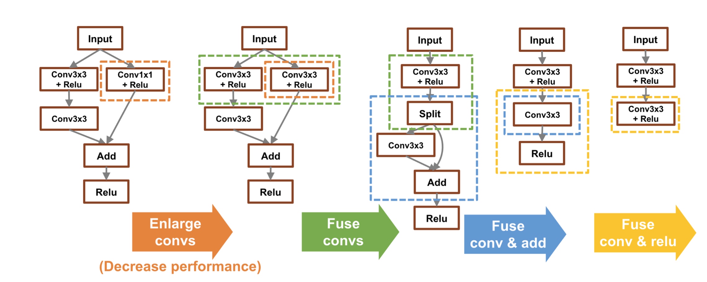
Graph Optimization
The goal is to rewrite the original graph \(G\) as \(G’\) that is faster.
Consider the following motivating example - Typically, convolution is followed by batch normalization. Instead of performing batch normalization, just update the weights in convolution to do everything in one step!
Note that some steps can become slower based on the hardware, but you get the general idea.
Similarly, in attention calculations, the code is typically written with a concatenated vector of queries, keys and values. This version is optimal - it can be understood with Arithmetic Intensity which the ratio of #operations and #bytes. For example, an addition operation has intensity of \(1/3\) (2 loads and one store). However, fusing multiple arithmetic operations reduces the loads and stores by bringing all variables into memory once, improving the arithmetic intensity.
So how do we optimize graphs?
We write rules or templates for opportunities to simplify graphs. There is also implementation of auto-discovering optimizations in the latest libraries, we shall study these.
Parallelization
The goal is to parallelize the graph computation over multiple devices. Note that devices can be connected with fast (memory communication NVLink) and slow connections (across GPUs), with up to 10x performance difference. Ideally, we do not want to describe partitioning rules for every new model that comes up. Based on these communication patterns, distributing the tasks is not an easy problem. So, we shall discuss how we partition the computational graph on a device cluster.
Runtime and Scheduling
How do we schedule the compute, communication and memory in a way that execution is as fast as possible, communication is overlapped with compute and is subject to memory constraints?
Operator Implementations
The goal is this layer is to get the fastest possible implementation of matmuls, for different hardware, different precision and different shapes.
NVIDIA releases a GPU every 2 years, and they have rewrite all operations every time! Notably, previously, models were trained using 32-bit floating points, but now researchers are emphasizing on lower and lower precisions.
Now, we shall delve into each of these architectures.
Operator Optimization and Compilation
The goal is maximize arithmetic intensity. In general there are three ways to speed up operators
Vectorization
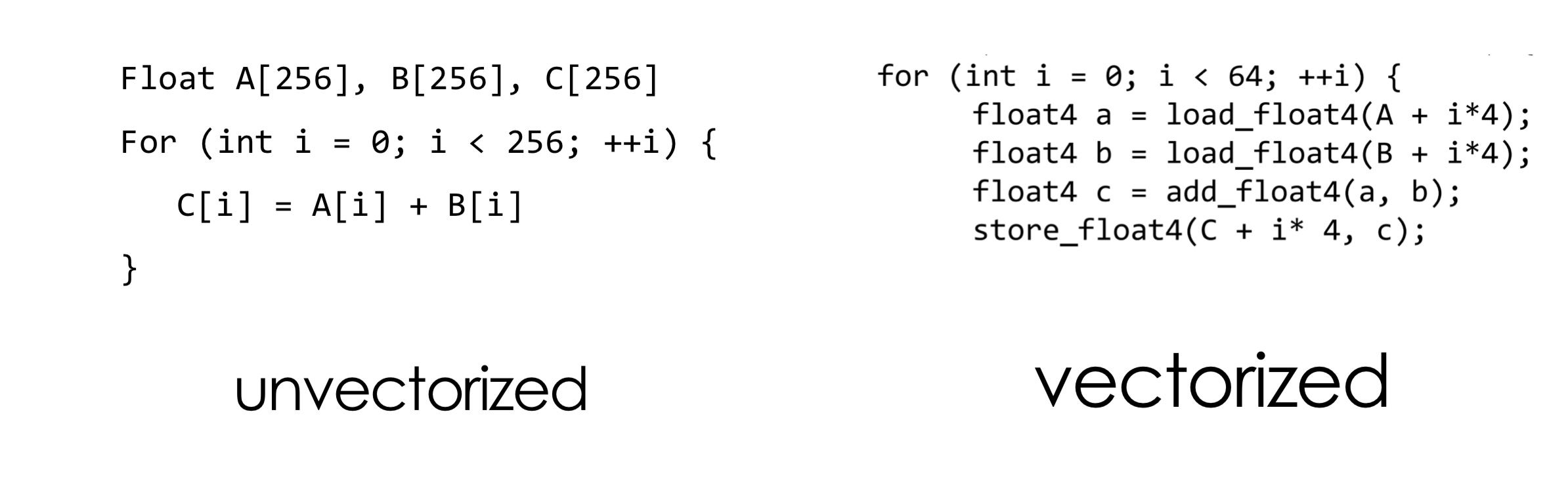
The right version is faster because of the hardware - cache sizes, etc. Tensorflow and PyTorch have this built-in.
Refactoring data layout
This is again related to how data is stored in memory. For example, C++ stores matrices in row-major order. Accessing columns of a matrix can be 10x slower! Remember this while writing code to lower cache misses and reduce pointer movements.
ML systems don’t store tensors in row or column major but in a new format called strides format - A[i, j, …] = A.data[offset + i*A.strides[0] + j*A.strides[1] + …. It is a generalization of row and column major storage, and it offers more flexibility - so based on the batch-sizes or other parameters in a neural network.
Strides can separate the underlying storage and the view of the tensor. Consider the following operations
-
slice- simply changing the offsets and shape will output the slice without any copying involved. -
transpose- modifying strides will transpose the tensor without any copying! For example, consider the following exampleM.strides() # (24, 12, 4, 1) M.permute((1, 2, 3, 0) M.t.strides() # (12, 4, 1, 24) -
broadcast- Suppose we have to extend a tensor’s data across a dimension for performing operations with another tensor, then by simply adding0stride in the appropriate dimensions would be enough! Again, no copying
Many more operations can be done without copying the data and simply modifying the strides. For example, consider the following example -
However, strides also has an issue - Memory access may become non-contiguous, and many vectorized ops require continuous storage.
Summary
To make operators efficient, we have seen the following tactics -
- Vectorization - leverage platform-specific vectorized functions that reduce seek time
- Data layout - strides format that allow zero-copies enabling fast array-manipulations
- Parallelization on CPUs
These were techniques for general operations. However, we can optimize certain operators with their special properties.
Matmul optimization
The brute-force approach takes \(\mathcal O(n^3)\). The best approach humans know is \(\mathcal O(n^{2.371552})\)!
How to improve the speed in practice then? Recall that we are trying to increase AI = #ops/#bytes.
Memory Hierarchy If everything ran on registers, things would be super-fast. But, that is expensive. Remember that L1-Cache has 0.5ns latency, L2-Cache has 7ns and DRAM has 200ns (400x slower!)
Let us analyze the AI of matmul considering the different layers of memory
- We can directly move data to registers in every iteration in inner loop
GPUs and accelerators
Recall that parallelizing operations across threads is super useful! CPUs have some level of parallelism through SIMD operations (vectorization) but they are limited. Building on the same idea, GPUs were born.
When we started out, the ALU units were limited by the physical space on the chips. As technology improved, we moved from 70nm process all the way 3nm process! That is, we can fit up to 20x more cores in the same area! The majority of the area on CPUs is consumed by Control and Cache, and Jensen thought, ditch those and put cores.
Graphical Processing Unit (GPU) are tailored for matrix or tensor operations. The basic idea is to use tons of ALUs (weak but specialized) with massive parallelism (SIMD on steroids).
There are other hardware accelerators like Tensor Processing Unit (TPU) or Application specific integrated circuit (ASIC), etc. The common theme across all these is the same - there are specialized cores. What are specialized cores? They can only compute certain computations. Specialized cores can be super powerful - 
Companies also tried reducing precision and maintain the same performance. Additionally, they also tune the distribution of different components for specific workloads.
Why does quantization work in ML systems?
Recap
Consider the following question - What is the arithmetic intensity of multiplying two matrices?
Load A
Load B
C = matmul(A, B)
Given \(A \in \mathbb{R}^{mxn}, B \in \mathbb{R}^{nxp}, C \in \mathbb{R}^{mxp}\), the number of I/O operations is \(mn + np + mp\), and the number of compute operations is \(2mnp\) since there are approximately \(mnp\) addition and multiplication operations. The arithmetic intensity is then \(\frac{\text{\#compute operations}}{\text{\#I/O operations}} = \frac{2mnp}{mn + np + mp}\). Setting \(m=n=p=2\), results in \(\frac{2x2x2x2}{2x2 + 2x2 + 2x2} = \frac{4}{3}\).
\textit{Note.} The addition operation discussed in the previous lecture also has the same I/O operations. However, \texttt{matmul} is a denser operation that results in a higher arithmetic intensity. In practice, it takes the same time to execute matrix addition and multiplication on GPUs, which is why they are so powerful.
matmul is an important operation.
Now, consider the following operations
broadcast_toslicereshape- Permute dimensions
transpose- indexing like
t[:, 1:5]
All these operations are optimized due to strided access in tensors. On the other hand contiguous() cannot take advantage of this.
Just to recap, the strides of a tensor of shape [2, 9, 1] stored in row major order are [9, 1, 1]
Consider the cache tiling operation -
- It increases the memory allocated on Cache and memory transfers between cache and register
- It reuses the memory movement between Dram and Cache
- The arithmetic intensity decreases since there is more load and store
GPU and CUDA
We have seen that specialized cores offer much better performance over traditional CPUs. Consider the following basic architecture of a GPU
Let us see the basic terminology for understanding the architecture -
- Threads - Smallest units to process a chunk of data.
- Blocks - A group of threads that share memory. Each block has many threads mapped to a streaming multiprocessor (SM/SMP).
- Grid - A collection of blocks that execute the same kernel.
- Kernel - CUDA program executed by many CUDA cores in parallel.
A GPU can be made more powerful by
- Adding SMs
- Adding more cores per SM
- Making the cores more powerful - at a point of diminishing rewards.
NVIDIA, the largest GPU company, has released P100, V100, A100, H100 and B100 (Blackwell) for ML development. K80, P4, T4 and L4 were a lower tier of GPUs. Let us analyze how the compute has changed across these versions
- V100 (2019 -) - 80SMs, 2048 threads/SM - $3/hour
- A100 (2020 -) - 108SMs, 2048 threads/SM - $4/hour
- H100 (2022 -) - 144SMs, 2048 threads/SM - $12/hour
- B100 and B200 (2025 -)-
The numbers are not doubling, then how has the performance doubled? They decreased the precisions.. :(
CUDA
What is CUDA? It is a C-like language to program GPUs, first introduced in 2007 with NVIDIA Tesla architecture. It is designed after the grid/block/thread concepts.
CUDA programs contain a hierarchy of threads. Consider the following host code -
const int Nx = 12;
const int Ny = 6;

dim3 threadsPerBlock(4, 3, 1); // 12
dim3 numBlocks(Ns/threadsPerBlock.x , Ny/threadsPerBlock.y , 1); // (3, 2, 1) = 6

// the following call triggers execution of 72 CUDA threads
matrixAddDoubleB<<<numBlocks, threadsPerBlock>>>(A, B, C);
The GPUs are associated with constants such as
-
GridDim- dimensions of the grid -
blocking- the block inter within the grid -
blockDim- the dimensions of a block -
threadIdx- the thread index within a block With these in mind, the CUDA kernel for the above code is designed as
    __device__ float doubleValue(float x)
    {
        return 2*x;
    }

    // kernel definition
    __global__ void matrixAddDoubleB(float A[Ny][Nx], float B[Ny][Nx], float C[Ny][Nx])
    {
        int i = blockIdx.x * blockDim.x + threadIdx.x;
        int j = blockIdx.y * blockDim.y + threadIdx.y;
        C[j][i] = A[j][i] + doubleValue(B[j][i]);
    }
The host code launched a grid of CUDA blocks, which then call the matrixAdd kernel. The function definition starts with __global__ which denotes a CUDA kernel function that runs of the GPU. Each thread indexes its data using blockIdx, blockDim, threadIdx and execute the compute. It is the user’s responsibility to ensure that the job is correctly partitioned and the memory is handled correctly.
The host code has a serial execution. However, the device code has SIMD parallel execution on the GPUs. When the kernel is launched, the CPU program continues executing without halting while the device code runs on the GPU. Due to this design, it is important that the device code does not have any return values - causes erroneous behavior. To get results from the GPU, CUDA.synchronize is used (an example will be shown later).
It is the developers responsibility to map the data to blocks and threads. The blockDim, shapes etc should be statically declared. This is the reason why compilers like torch.compile requires static shapes. The CUDA interface provides a CPU/GPU code separation to the users.
The SIMD implementation has a constraint for the control flow execution - it requires all ALUs/cores to process in the same pace. In a control flow, not all ALUs may do useful work and it can lead to up to 8 times lower peak performance.
Coherent and Divergent execution
A coherent execution applied the same instructions to all data. Divergent executions do the opposite and they need to be minimized in CUDA programs. This distinction is important to note - even the latest models like the LLMs have this behavior. Concepts such as attention masking and sliding window attention are examples of divergent behavior and they need to be specially implemented to extract the most compute from the GPU.
CUDA Memory model
CUDA device (SIMD execution on GPU) has its own memory called the HBM.
Unlike host (CPU) memory that is stored as pages in the RAM, GPU memory does not use pages but has memory pools (bulk data) that are accessed all at once.
Memory can be allocated cudaMalloc and populated with cudaMemcpy like usual. CUDA has a concept called pinned memory that is part of the host memory which is optimized for data transfer between CPU/GPU. Ig is not pagable by the OS and is locked, and only certain APIs can access it.
Every thread has its own private memory space, and every block has a shared memory that all its threads can access. The HBM is the global device memory in the GPU that can be accessed by all threads. The memory complexity is to balance between speed and shared memory parallelism.
For example, consider the program for window averaging -
    for i in range(len(input) - 2):
        output[i] = (input[i] + input[i + 1] + input[i + 1])/3.0
How can this be parallelized? Since every 3-element tuple reduction is independent, each reduction can be mapped to a CUDA core. So, each thread can compute the result for one element in the output array.
The host code -
int N = 1024*1024;
cudaMalloc(&devInput, sizeof(float)*(N+2)); // To account for edge conditions
cudaMalloc(&devOutput, sizeof(float)*N);

convolve<<<N/THREADS_PER_BLK, THREADS_PER_BLK>>>(N, devInput, devOutput);
The device code -
    #define THREADS_PER_BLK = 128

    __global__ void convolve(int N, float* input, float* output) {
        int index = blockIdx.x *blockDim.x + threadIdx.x;
        float result = 0.0f; //thread-local variable
        result = input[index] + input[index + 1] + input[index + 2];
        output[index] = result /3.f;
    }
This program can be optimized - each element is read thrice!
Notice that the number of blocks assigned is much more than what a typical GPU has. This is a general practice in CUDA programming where the blocks are oversubscribed.
How to optimize? The memory hierarchy can be utilized -
The new device code -
   #define THREADS_PER_BLK = 128

    __global__ void convolve(int N, float* input, float* output) {
        int index = blockIdx.x *blockDim.x + threadIdx.x;

        __shared__ float support[THREADS_PER_BLK];
        support[threadIdx.x] = input[index];
        if(threadIdx.x < 2){
            support[THREADS_PER_BLK + threadIdx.x] = input[index + THREADS_PER_BLK];
        }

        __syncthreads();

        float result = 0.0f; //thread-local variable
        for(int i=0; i<3; i++)
            result += support[threadIdx.x + i];

        output[index] = result /3.f;
    }
We introduced a synchronization primitive here. _syncthreads() waits for all threads in a block to arrive at this point. Another primitive cudasynchronize() that syncs between host and the device.
Compilation
A CUDA program also needs to be converted to low-level instructions to be executed. A compiled CUDA device binary includes -
- Program text (instructions)
- Information about required resources - 128 threads per block, 8 types of local data per thread and 130 floats (520 bytes) of shared space per thread block.
The issue is that different GPUs have different SMs. If the user asks for a static (large) number of blocks, how to handle this? The first solution is that GPUs have varying (limited) number of blocks.
Furthermore, CUDA schedules the threadblocks to many cores using a dynamic scheduling policy that respects the resource requirements. It assumes that the thread blocks can be executed in any order. The blocks are assigned based on the available resources and the remaining ones are queued.
Understanding a GPU
Consider a NVIDIA GTX 980 (2014) that has the following specs -
- 96KB of shared memory
- 16 SMs
- 2048 threads/SM
- 128 CUDA cores/SM Note that the number of CUDA cores is not equal to the number of CUDA threads.
As the GPUs became better, NVIDIA tried to increase the shared memory per SMM. This is similar to the SRAM which is very important for LLM inference.
matmul - Case Study
Remember that over subscribing in GPUs is allowed, and identify that work can be performed in parallel. Developing the thought-process while working with CUDA is important
- Oversubscribe to keep the machine busy
- Balance workload with convergent workflows
- Minimize communication to reduce I/O
Now, let us consider matrix multiplication. What can be parallelized? In our previous CUDA implementation, we let each thread compute one element in the result matrix. So, each thread has \(2N\) reads, and there are \(N^2\) threads, resulting in \(2N^3\) global memory access.
We are not leveraging the fact that one element can be used to calculate many values in the result matrix. The trick is to use the shared memory space - thread tiling (similar to what we did in CPUs).
We let each thread compute \(V \times V\) submatrix. The kernel is as follows
    __global__ void mm(float A[N][N], float B[N][N], float C[N][N]) {
        int ybase = blockIdx.y * blockDim.y + threadIdx.y;
        int ybase = blockIdx.y * blockDim.y + threadIdx.y;

    float C[V][V] {0};
    float a[N], b[N];
    for (int x = 0; x < V; ++x){
        a[:] = A[xbase * V + x, :];
        for (int y = 0; y < V; ++y){
            b[:] = B[:, ybase * V + y];
            for (int k = 0; k < N; ++k){
                c[x][y] += a[k]*b[k];
            }
        }
    }
    C[xbase * V: xbase*V + V, ybase * V: ybase*V + V] = c[:];
}
For this version, we have reduced the read per threads to \(NV + NV^2\) and number of threads to \(N^2/V^2\) - total reads reduce to \(N^3/V + N^3\) with \(V^2 + 2N\) float storage per thread.
We can improve this using partial sum computations. With a small change, we get
    __global__ void mm(float A[N][N], float B[N][N], float C[N][N]) {
        int ybase = blockIdx.y * blockDim.y + threadIdx.y;
        int ybase = blockIdx.y * blockDim.y + threadIdx.y;

    float C[V][V] {0};
    float a[N], b[N];
    for (int k = 0; k < N; ++k){
        a[:] = A[xbase * V: xbase * V + V, k]; // Grabbing an area
        b[:] = B[k, ybase * V:ybase * V + V];
        for (int y = 0; y < V; ++y){
            for (int x = 0; x < V; ++x){
                c[x][y] += a[x]*b[y];
            }
        }
    }
    C[xbase * V: xbase*V + V, ybase * V: ybase*V + V] = c[:];
}
With memory read per thread reduced to \(NV^2\), total memory to \(2N^3/V\) and memory per thread to \(V^2 + 2V\). This version is pretty good for systems with a single layer of memory hierarchy. However, if we have shared memory, it can be made more efficient!
Suppose we have an SRAM layer, we can tile hierarchically. Consider the following GPU matmul v3: SRAM Tiling:
The idea is to use block shared memory to let a block compute a \(L \times L\) submatrix and each thread computes a \(V \times V\) submatrix reusing the matrices in the shared block memory.
    __global__ void mm(float A[N][N], float B[N][N], float C[N][N]) {
    __shared__ float sA[S][L], sB[S][L];
    Float c[V][V] = {0};
    Float a[V], b[V];
    Int y block = blockIdx.y;
    Iint X block = blockIdx.x;
        int ybase = blockIdx.y * blockDim.y + threadIdx.y;
        int ybase = blockIdx.y * blockDim.y + threadIdx.y;

    float C[V][V] {0};
    float a[N], b[N];
    for (int k = 0; k < N; ++k){
        a[:] = A[xbase * V: xbase * V + V, k]; // Grabbing an area
        b[:] = B[k, ybase * V:ybase * V + V];
        for (int y = 0; y < V; ++y){
            for (int x = 0; x < V; ++x){
                c[x][y] += a[x]*b[y];
            }
        }
    }
    C[xbase * V: xbase*V + V, ybase * V: ybase*V + V] = c[:];
}
Think about it this way. Initially, we performed tiling across one layer of memory balancing the tradeoffs between I/O reads and memory constraints of the threads. Now, we are adding one more layer of such tiling in a similar manner. The key is to understand the partial sums idea.
Note that it is highly unlikely that the threads have a large range of execution times, but we have the __syncthreads() as a failsafe. The statistics of this algorithm are -
- \(2LN\) global memory access per thread block
- \(N^2/L^2\) threadblocks
- \(2N^3/L\) global memory access
- \(2VN\) shared memory access per thread
The key addition here is was the shared memory space. For this algorithm to be efficient, the fetching from the memory has to be implemented cooperatively -
    int nthreads = blockDim.y * blockDim.x;
    int tid = threadIdx.y * blockDim.x + threadIdx.x;
These summarize the matrix multiplication codes implemented in the GPUs. Simple, isn’t it? Although, we have not addressed the optimal values for \(L, V\). It depends on the number of threads, registers and amount of SRAM available on the GPU - this process is called kernel tuning. There are profilers that optimize these values. It is a difficult problem since large ML models have various operations that need to be optimized together based on their processing and memory requirements. Furthermore, this is different for every GPU and there are hundreds of GPUs!
One solution is to do brute-force - hire people and throw money at it. On the other side of things, ML researchers are building operator compilers that figure these out automatically.
There are other GPU optimizations that are utilized in practice
- Global memory continuous read
- Shared memory bank conflict
- Pipelining - While some threads are reading, let other threads compute.
- Tensor core - Dedicated hardware component to accelerate matrix multiplications
- Lower precisions
ML compilation
A super-hot topic during the late 2010s since there was a lot of inefficient code that was being identified. The goal is to automatically generate optimal configurations and code given users code and target hardware.
Traditional compilers have to simply convert high-level code to binary instructions. The stack for ML compilers is
- Dataflow graph generation
- Optimize graphs - pruning, partitioning, distribution, etc
- Build efficient kernel code - parameter optimization
- Machine code (This step is fairly easy and already well implemented)
The big problems in this big process are
- Programming level - Automatically transforming arbitrary (usually imperative) code into a compilable code (static dataflow graphs)
- Graph level - Automatic graph transformations to make it faster (recall how convolution and batch norm can be fused). Graph theory researchers are working on this.
- Operator level - How to use hardware and optimize standard operators like
matmul.
The big players in this big field are
- XLA - First compiler for ML, released along with TensorFlow in 2016 (those researchers aimed big). This turned out to be so good, that the current TensorFlow stack still uses this. Also works for PyTorch, and it is useful to deploy on TPUs.
- tvm (Tensor Virtual Machine) - It is one of the most successful open-source compiler in academia. They founded OctoML with 200M (got acquired by NVIDIA). There is no backward pass.
- 2.0 - Torch based compiler, that isn’t that great in terms of optimization.
- Modular - They raised 300M, founded by the same person who created LLVM. The co-founders started swift at Apple! They had big claims - 20x faster than 2.0, not sure how true they are.
You can think of TensorFlow and PyTorch as the front end, and the above mentioned compilers as the backend.
Operator Compilation
Each user-level written code (for standard operations) has a library of low-level program variants, and the compiler chooses the fastest one for the given hardware.
For example, consider a loop -
    for x in range(128):
        C[x] = A[x] * B[x]
Get converted to
for xi in range(4):
    for xo in range(32):
        C[xo * 4 + xi] A[xo * 4 + xi] + B[xo * 4 + xi]
Which is then efficiently implemented in the GPU kernels.
So, how do we make this happens?
- Enumerate all possibilities
- Enumerate all the (close-to-) optimal values for the hardware - register/cache
- Apply to all operators and devices
How to search or reduce the search space and generalize?
Note that for a certain kind of code and hardware, finding these optimal value once is enough.
Search via Learned Cost Model
The famous example is Autotvm -
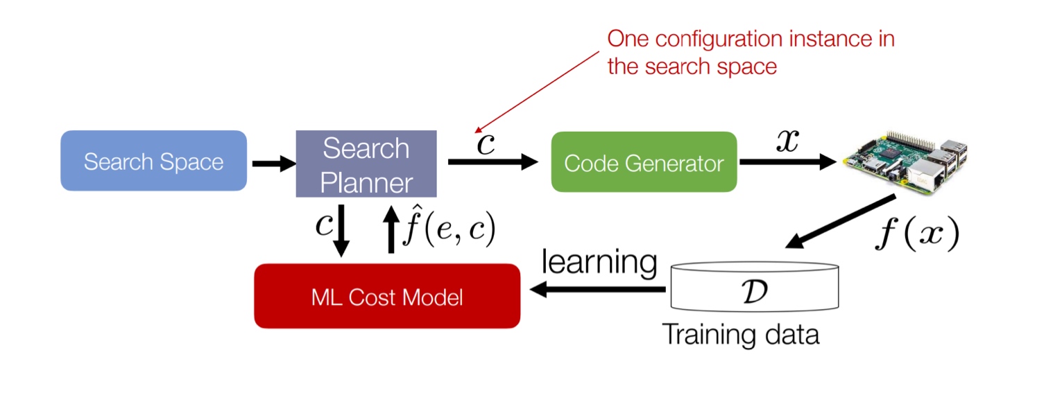 The code generator here is done with templates (not LLMs).We need a lot of experts to write the template to define the search space.
To search in this parameters space, the compiler does beam search with early pruning. The cost model can be trained on the historical data.
High-level ideas
We represent the programs in an abstract way and build a search space with a set of transformations (that represent a good coverage of common optimizations like tiling). Then effective search with accurate cost models and transferability have to be deployed.
So, how well are we doing in this field? If the compilers were that good, they would’ve discovered flash-attention. Okay, it’s not that bad, compilers have found good optimizations and it just goes to show how difficult this problem is.
High-level DSL for CUDA: Triton
We have seen a device-specific DSL (domain-specific language). Programmers are able to squeeze the last bits of performance through this. However, it requires deep expertise and the performance optimization is very time-consuming. Maintaining codebases is complex.
On the other hand, we have ML compilers. They prototype ideas very quickly (automatically) and the programmer does not have to worry about the low-level details. The problem is representing and searching through the search-space is difficult. Compilers were not able to find Flash-attention because the search-space wasn’t able to represent this possibility. Furthermore, code generation is a difficult problem that relies on heavy use of templates - lots of performance cliffs.
So compared to these two extremes, Triton is in between - it is simpler than CUDA and more expressive than graph compilers. It was developed by OpenAI as a solution to the problems with CUDA and compilers.
Triton Programming Model
The users define tensors in SRAM directly and modify them using torch-like primitives.
- Embedded in Python - Kernels are defined in Python using triton.jit
- Supports pointer arithmetics - Users construct tensors of pointers and can (de)reference them element wise.
- However, it has shape constraints - must have power-of-two number of elements along each direction
Consider the following example
    import triton.language as tl
    import triton

    @ triton.jit
    def __add(z_ptr, x_ptr, y_ptr, N)
        offsets = tl.arange(0, 1024)
The triton kernel will be mapped to a single block (SM) of threads. The users are responsible for mapping to multiple blocks. Basically, the language is automating some parts (like compilers), and making the design process simpler for users (as compared to CUDA). These design philosophies are important because they help build newer mental models for users - because they offload some of the cognitive load for optimization, they can think of newer ways of optimizing with these restricted set of parameters. Consider the example of softmax calculation. This function would be slow if implemented using primitives. PyTorch implements an end-to-end kernel for softmax to increase its performance. With triton, we can construct such an end-to-end operation in a simpler manner while achieving slightly higher performance.
import triton.language as tl
import triton
@triton.jit
def _softmax(z_ptr, x_ptr, stride, N, BLOCK: tl.constexpr):
    # Each program instance normalizes a row
    row = tl.program_id(0)
    cols = tl.arange(0, BLOCK)
    # Load a row of row-major X to SRAM
    x_ptrs = x_ptr + row*stride + cols
    x = tl.load(x_ptrs, mask = cols < N, other =    float(‘-inf’))
    # Normalization in SRAM, in FP32
    x = x.to(tl.float32)
    x = x - tl.max(x, axis=0) # This is to avoid vert large and small values
    num = tl.exp(x)
    den = tl.sum(num, axis=0)
    z = num / den;
    # Write-back to HBM
    tl.store(z_ptr + row*stride + cols, z, mask = cols < N
Note that Triton achieves good performance with low time investment. However, since it is not as flexible as CUDA, achieving very high-performance is not possible with Triton.
Recap
A kernel in the GPU is a function that is executed simultaneously by tens of thousands of threads on GPU cores. The shared memory during the GPU execution can be used as a cache that is used by more than one thread, avoiding multiple accesses to the global memory. Over-subscribing the GPU ensures that there are more blocks than SMPs present on the device, helping to hide (tail) latencies by ensuring high occupancy of the GPU.
<iNsert a point about GPU memory)
Operations such as ReLU, batch normalization and max pooling are not arithmetically dense operations. So typically, operations such as linear layers (and layer normalization with large batches) are limited by arithmetic operations. To calculate which linear layer would have more operations, consider the FLOPs calculation for GEMM.
(3) Graph Optimization
Our goal is to rewrite \(G\) as \(G’\) such that \(G’\) runs faster than \(G\) while outputting equivalent results. The straightforward solution is to use a template, wherein human experts write (sub-)graph transformation templates and an algorithm replaces these in the data flow graphs for reduction.
Graph Optimization Templates: Fusion
Fusing operators reduces I/O and kernel launching (CPU to GPU overhead, all the operations that the SM has to run). The disadvantages of this method is that creating various fused operations is difficult making the codebase unmanageable (e.g., TensorFlow).
This also includes folding constants in a graph to replace expressions such as (X + 3) + 4) with (X + 7).
CUDA graph
NVIDIA allows users to capture the graph at the CUDA level.

Is this define-then-run?
Standard compiler techniques
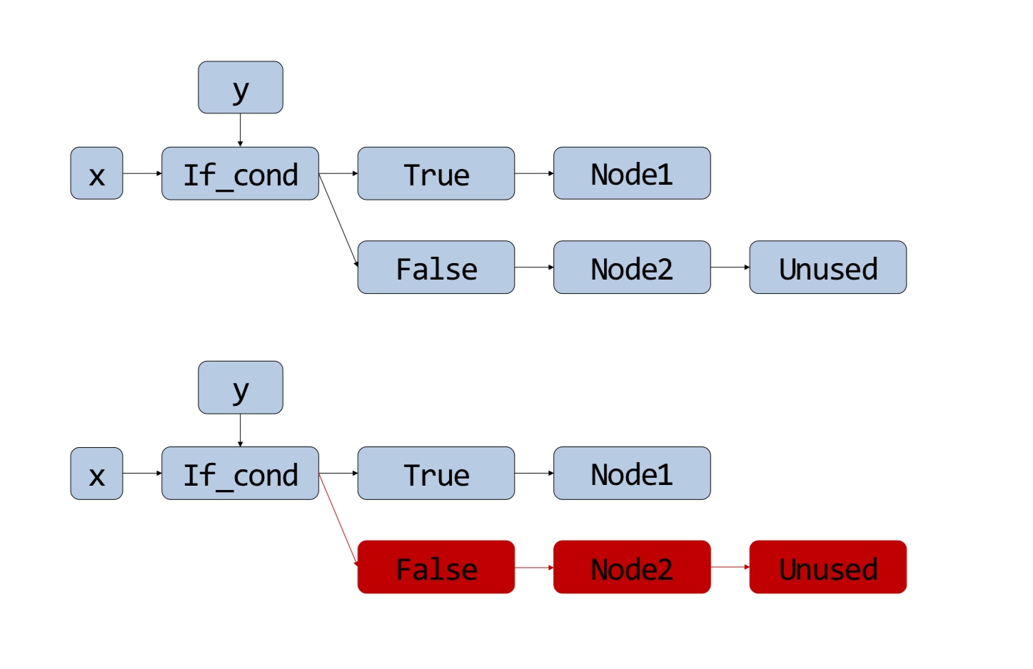
- Common subexpression elimination (CSE). The high-level idea is replacing expressions such as
a = b; b = cwitha = c - Dead Code elimination (DCE). After the CSE hit, we eliminate the dead-code with unused variables.
These both are run iteratively to reach an optimal code. These operations are every useful to eliminate parts of graph based on, say default arguments -
How to ensure performance gain?
When we greedily apply graph optimizations, we may miss some options that initially decrease the performance but massively increase it later. Furthermore, the same optimizations could lead to an improvement in one hardware and reduction in other. Due to the existence of hundreds of operators (200-300), thousands of graph architectures and tens of hardware backends, it is infeasible to manually design graph optimizations for all cases.
There are other issues with template based optimizations
- Robustness - Heuristics are not generalizable across architectures and hardware
- Scalability - New operators and graph structures require newer rules
- Performance - Misses subtle optimizations specific to DNNs/hardware.
What’s the solution?
Automate Graph Transformation
The main idea is to replace manually-designed graph optimizations with automated generation and verification of graph substitutions for tensor algebra. Basically, generate all possible substitutions and verify if they generate the same output.
We start by enumerating all possible graphs up to a fixed size using available operators.
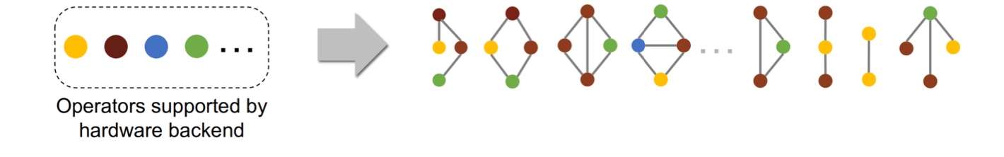 There are up to 66M graphs with 4 operators!
Then, with a graph substitution generator, we compute the output with random input tensors. For 4 operators, we can still generate up to 28744 substitutions!
These are further pruned based on variable renaming and common subgraphs.
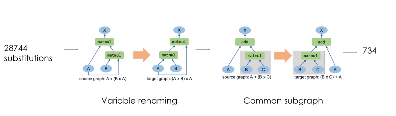
These substitutions are formally verified to ensure that they are equivalent mathematically for all inputs. This verification is done by using the properties of operators. For example, convolution with concatenated kernels is same as concatenation of convolutions of the same kernels.
So this automated theorem prover can be used to generate valid substitutions scaling up. It takes up to 5 minutes to verify 750 substitutions and there are about 45 rules for the operators which takes about 10 minutes. Adding a new operator is easy - just provide its specifications!
Incorporating substitutions
How do we apply verified substitutions to obtain an optimized graph? The cost is based on the sum of individual operator’s cost and the cost on the target hardware. We greedily apply the substitutions to improve the performance.
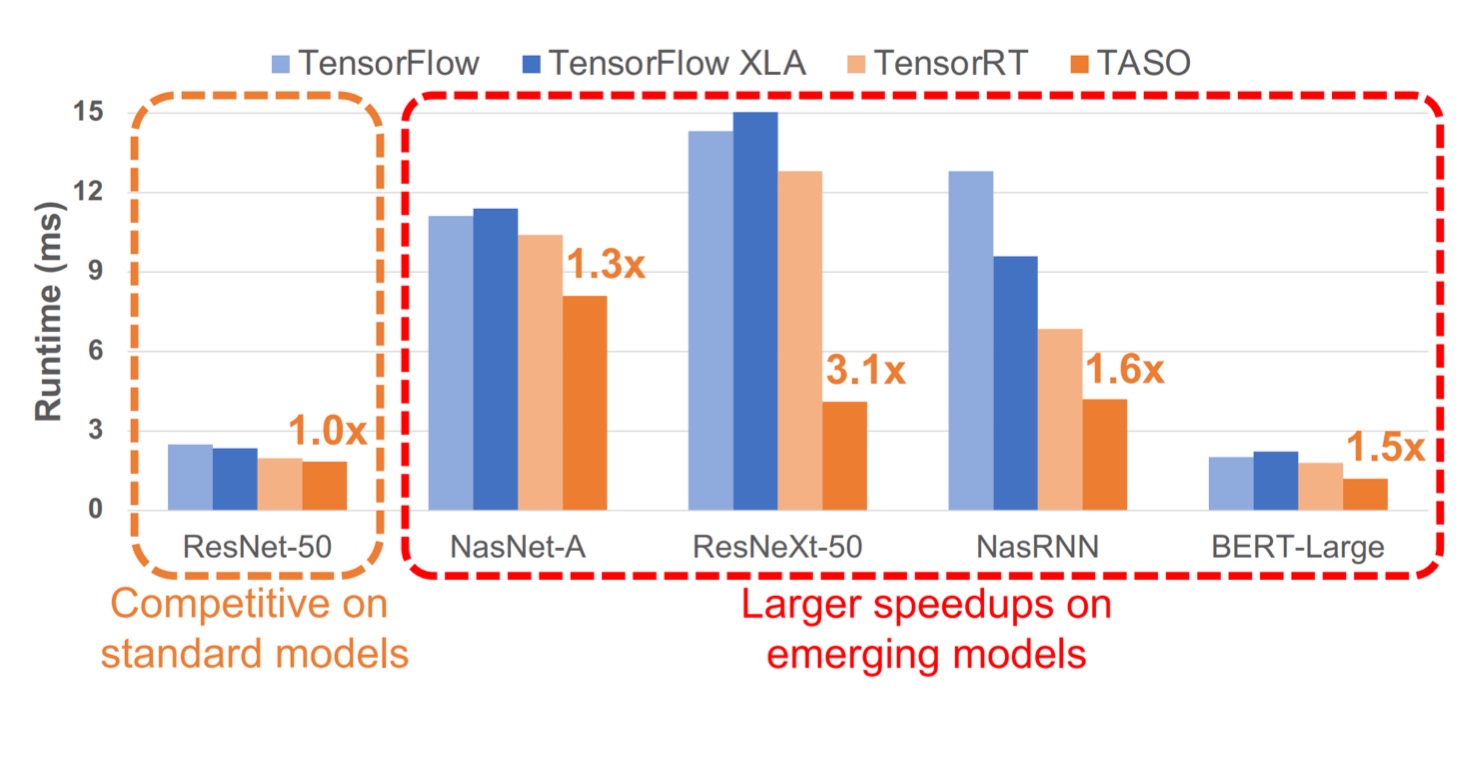
This approach can be further improved to train a model to learn which kind of substitutions optimize the graph. This was successfully implemented by TASO and it showed good results for real-life models -
Summary
In summary for graph optimization,
- We first construct a search space
- Enumerate all possibilities for substitutions
- Prune the candidates, and select the top ones based on profile/cost model
- Apply the transformations to iteratively improve the performance.
What could go wrong with this? The search may be slow and the evaluation of various graphs can be expensive.
Sometimes the substitutions may only be partially equivalent, but can be orders of magnitude faster. In such cases, we can trade off accuracy for performance. E.g., Convolution vs Diluted convolution.
Consider the following example. Suppose we have to use the same kernel to perform convolution on two different tensors. Then, we could concatenate these tensors, apply the convolution, and then apply a correction to achieve the correct result. These transformations use partial equivalent transformations yielding some speed up. These are not explorable in the previous case with fully equivalent operators.
Partially Equivalent Transformations
Like the previous example, we mutate the programs and correct them to get an optimized graph.
The steps to do this automatically, we do something similar to before
- Enumerate all possible programs up to a fixed size using available operators
- Only consider transformations with equal shapes (in contrast with equal results as compared to before)
With this, all the crux of the algorithm comes to the correction of the mutant programs - how do we detect which part is not equivalent and how to correct it?
By enumeration - For each possible input and position, check if the values match. For complete correctness, this search would be \(m \times n\) for \(m\) possible inputs and \(n\) output shape. We reduce the effort by reducing \(m, n\)
-
Reducing \(n\) - Since neural networks are mostly multi-linear, we can make such assumptions.
Theorem: For two multi-linear functions \(f\) and \(g\), if \(f = g\) for \(O(1)\) positions in a region, then \(f = g\) for all positions in the region.
As a consequence, the search reduces from \(\mathcal O(mn)\) to \(\mathcal O(mr)\)
-
Reducing \(m\) - Theorem - If \(\exists l, f(l)[p] \neq g(l)[p]\), then the probability that \(f\) and \(g\) give identical results on \(t\) random inputs is \(2^{-31t}\).
Using this, we can run \(t\) random tests with random inputs, and if all \(t\) pass then it is very likely that \(f\) and \(g\) are equivalent.
The search space reduces to $\mathcal O(tr)$$. How does this relate to correct?
ML Compiler Retrospective
This field started in 2013 with Halide. It was a compiler for rendering, but since the workflow is very similar to neural networks, the later compilers draw motivation from here.
Then came XLA in 2016-17, that has good performance but had very difficult to understand code. Companies tried other operations such as TensorRT, cuDNN and ONNX for template based graph substitution. CuDNN is still popularly used but no one understands the code since it was written in a very low level language.
Then came tvm in 2018 that we’ve discussed before. In 2019-20, MLIR and Flexflow were introduced - these are layers in the compiler that provided specific optimizations. Then came 2.0 and Torch Dynamo.
However, the community is shifting away from compilers. Why? One part is that many optimizations have been found. The main reason is that we’ve seen a certain class of neural networks architectures that work really well. For example, transformers are all the rage. So instead of focusing on compilers, people can focus on just building fused kernels for the attention mechanisms. That’s how we got flash-attention that no compiler is able to beat.
Runtime
Memory and Scheduling
Our goal is to fit the workload on limited memory and ensure that the peak memory usage is less than the available memory.
Need to add some stuff here.
Consider the GPT-3 architecture -

For every model, we check the precision and multiply the number of parameters by 2 or 4 to calculate the total memory consumption.
For the main model with 175B parameters, if each parameter is 2 bytes, then we require 350Gb of memory! How did we make this work?
Why does this rule of thumb work? Let us check the activation sizes for different layers
- For 2D convolution: The input has the size \((bs, nc, wi, hi)\), and the output has \((bs, nc, wo, ho)\). The activation size is \(bs*nc*wo*ho*\text{sizeof(element)}\)
- For an MLP with input size \((bc, m, n)\) and output size \((bs, m, p)\), the activation size is \(bs*m*p*\text{sizeof(element)}\)
- For a transformer (ignoring activation layers and other FFLs) - the input size is \((bs, h, seq\_len)\) and the output size is \((bs, h, seq\_len). The activation size is\)bshseq_len*\text{sizeof(element)}$$
So for GPT-3, the per-layer activation assuming sequence length 1 comes to 78 or 156 Gb. Let us add some more elements to this calculation.
The Adam Optimizer estimates the first and second moment vectors with parameters for exponential decays. It also has a step-size or learning rate. The algorithm is given by
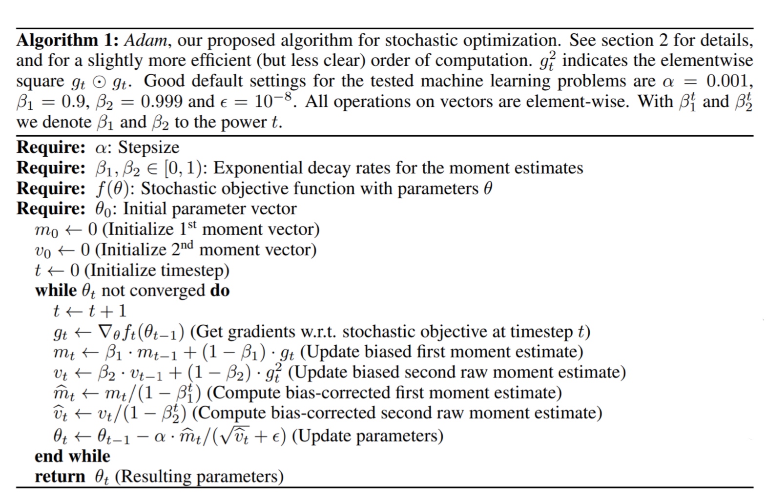
Along with the learning rate, since it also stores the moments, it has to store two more values for each parameter! The memory usage becomes thrice of what it should be!
Lifetime of activations at training
Because we need to store the intermediate values for the gradient steps, training an \(N\)-layer neural network would require \(O(N)\) memory. This is the main difference between training and inference. In inference, we wouldn’t need to store the parameters at all layers, so we would just need \(O(1)\) memory.
So we’ve seen for GPT-3, we require 350 or 700 Gb. So for a sequence length of 96, we would require 7488 or 14976 Gb! These numbers are just crazy! We haven’t even considered the composite layers.
Therefore, it is important to take care of memory.
Single Device execution
How do we reduce the memory usage?
Idea 1 - the input or the activation is not needed until the backward pass reaches the layer. So, we can discard some of them and recompute the missing intermediate nodes in small segments. This technique is called recomputation, rematerialization, checkpoint activation, etc. It’s essentially the time-space tradeoff.
For an \(N\) layer neural network, if we checkpoint every \(K\) layers, then the memory cost reduces to
\[\text{Memory cost} = \mathcal O\left(\frac{N}{K}\right) + \mathcal O(K)\]To minimize this, we can pick \(K = \sqrt{N}\). The total recomputation increases by \(N\) - essentially another forward pass. In PyTorch, this feature can be activated using torch.utils.checkpoint.
So when do we use this? When memory is a constraint and time of training is not a concern. The memory usage also depends on the layer being checkpointed - the layers can have different out sizes. In transformers, the layer boundary is typically checkpointed. The disadvantage is that this only works for activations.
why?
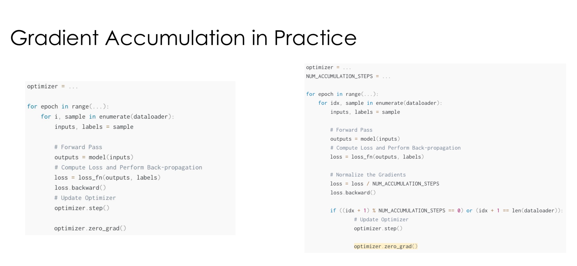
The second idea is gradient accummulation. The activation memory is linear to batch size. The idea is to compute the gradient for the batch but will limited memory. We split the original batch into micro-batches and accumulate the gradients at each layer. We then update the weights for the complete batch.
The disadvantage of this strategy is that over-subscribing of GPUs is difficult since we have smaller matrices.
An alternative method to save on GPU memory is to use the memory hierarchy. We have SwapIn (swap from CPU DRAM to HBM) and SwapOut (swap from HBM to CPU DRAM) that can be applied to both weights and activation. As we do a forward pass, we swap in the next layers and swap out the passed layers. You can be a bit more intelligent about it and pre-fetch the layers based on the computation and swap latencies. This strategy is becoming more practical as more companies are adopting the unified memory architecture. The memory hierarchy seems to be breaking.
All these strategies can be used together to probably train GPT-3 on a single device but it would take forever.
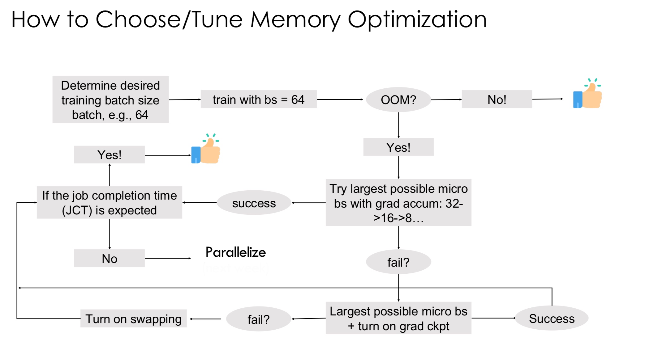 Why do we start with gradient accumulation instead of gradient checkpointing? Checkpointing greatly increases the computation time, so we try the other alternatives first.
Memory and Compute
Quantization
All our memory usage is a multiple of \(\text{sizeof(element)}\). What if we reduce that parameter?
Quantization is the process of constraining an input from a continuous or otherwise large set of value to a discrete set. We use a lower-precision representation for data while preserving ML performance (accuracy), speeding up compute, reducing memory, saving energy, etc. Most of the edge models use quantization.
To understand this better, let’s understand the representation of data in memory -
- An unsigned integer has the range \([0, 2^n - 1]\)
- A signed integer with \(n\)-bit has the range \([-2^{n-1} - 1, 2^{n - 1} - 1]\). To avoid saving 0 twice by storing a sign bit, computer architects decided to use Two’s complement representation.
- Fixed point number - An arbitrary bit is chosen as the boundary for the integer and the decimal. This representation is mainly used in security applications now.
-
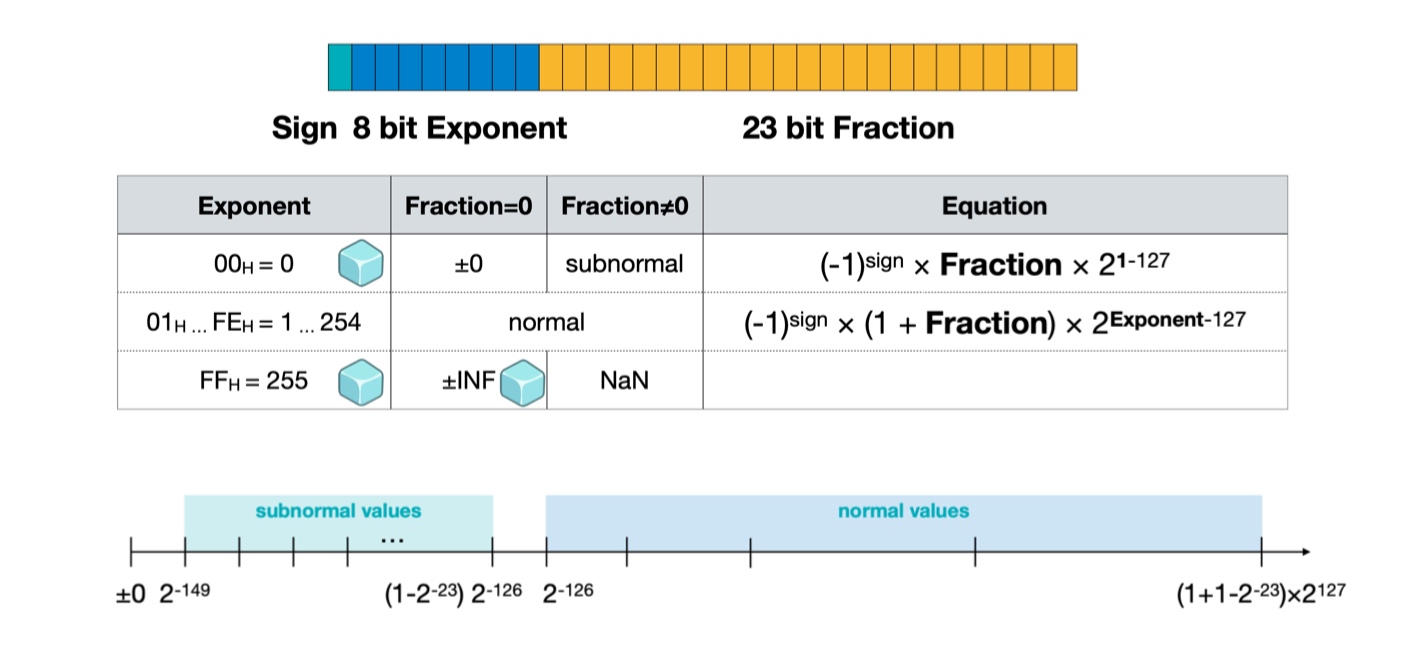
Floating point representation - We use a sign bit, 8-bit exponent and 23 bit fraction. That is the value is, \((-1)^{sign} \times (1 + \text{ fraction}) \times 2^{\text{exponent} - 127}\).
How do we represent 0 then? Representation-wise, we technically cannot represent 0, so we make a special representation - normal vs subnormal values. Whenever the exponent bits are zero, we remove the bias term \(1\) that is added to the fraction, and represent the value as \((-1)^{sign} \times \text{ fraction} \times 2^{\text{exponent} - 127}\). This expressions is only used with the exponent is \(0\). This way, we also extend the range of the representation and the smallest positive number we can represent is \(2^{-149}\).
How about special values? Exponent with all set bits is infinity and sign is decided by the sign bit. NaN is represented in the subnormal range with exponent bits set to 1. In summary, we have
Calculate model sizes from parameters table.
Notice that the precision of floating point numbers is much higher when the values themselves are small. This is a tradeoff we make based on the applications. Here is a summary of other floating point representations -
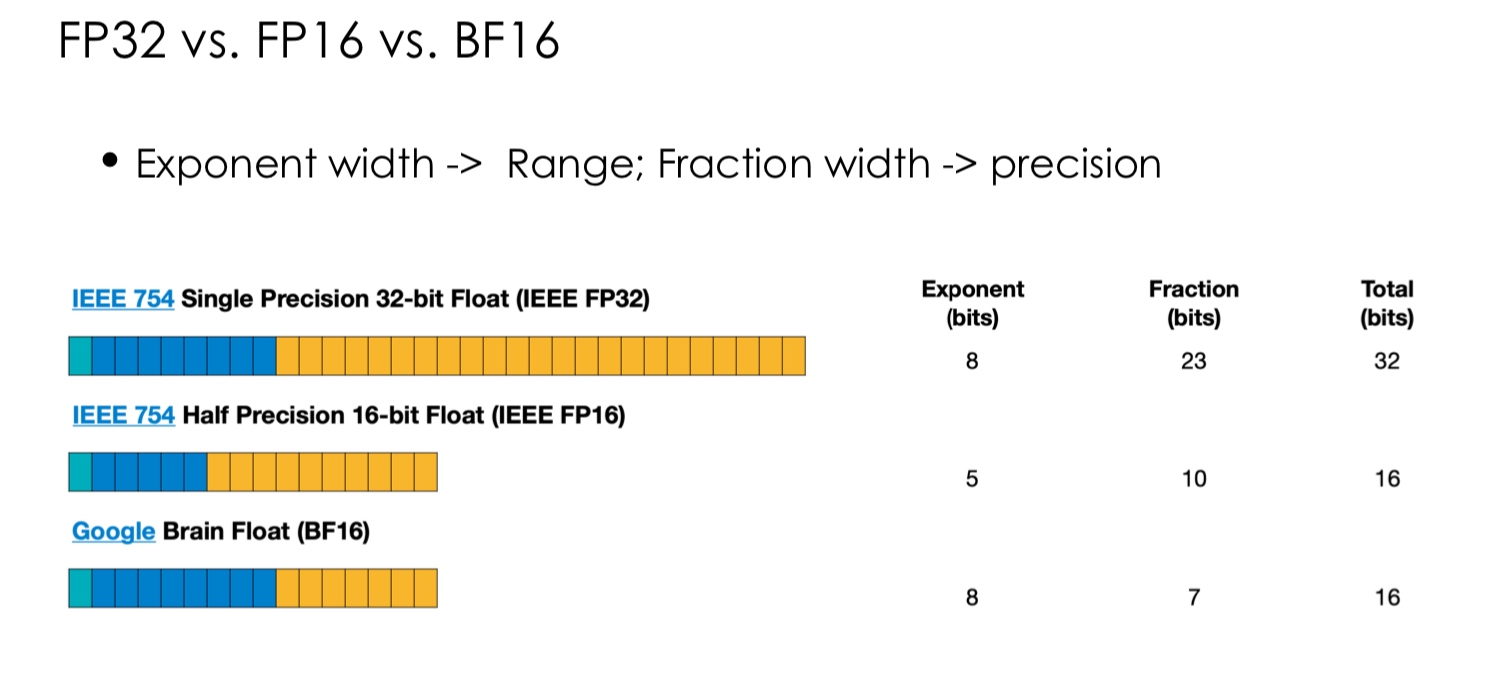
The BF16 system has been observed to provide much better performance over FP16 for neural network training. The representation lowers the precision for a higher range. It could be that the higher range can stabilize the training during exploding or vanishing gradients. During inference, the precision matters more so FP16 might perform better in some cases.
For practice, consider the following examples
- The FP16 bit set
1 10001 1100000000represents -7.1. Why? The bias in the exponent is always the median value subtracted by 1. Here it is \(2^4 - 1 = 15\). The exponent is then \(17 - 15 = 2\), and the fraction is \(0.5 + 0.25 = 0.75\) - The decimal 2.5 is represented as
0 10000000 0100000. The bias is \(2^7 - 1 = 127\)
After these representations, newer ones came up to improve the performance in deep-learning. 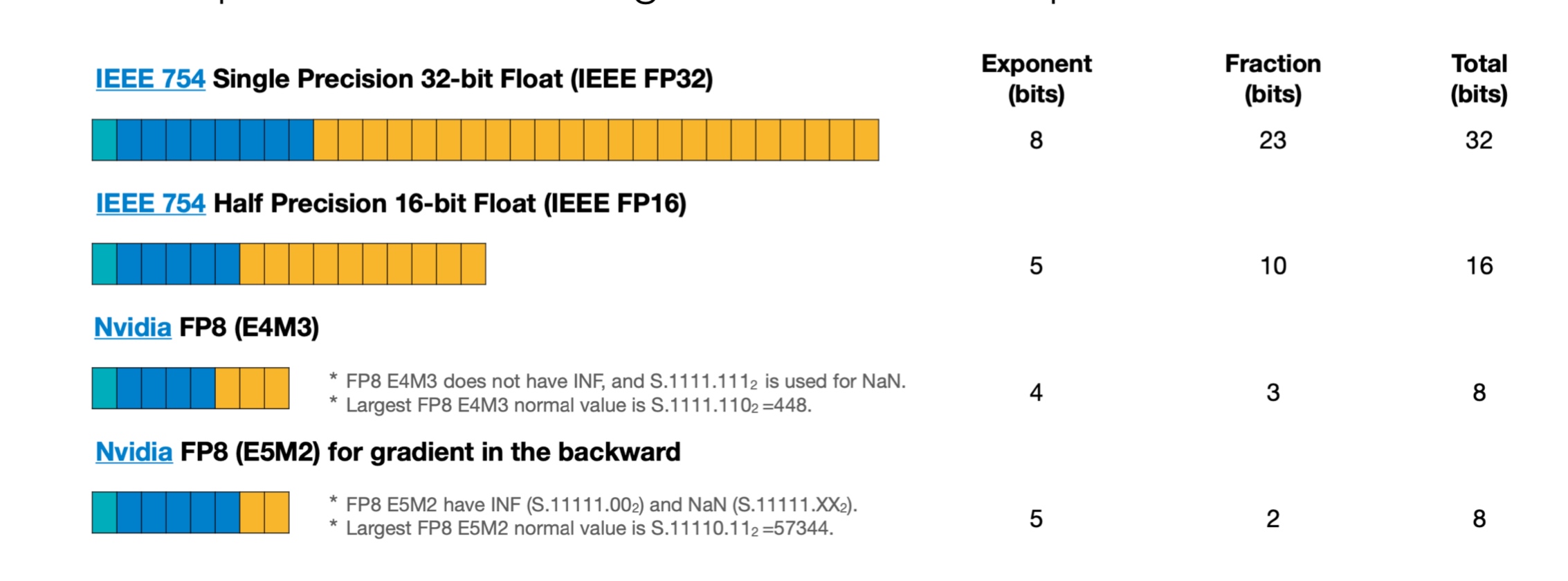 The rule of thumb is that we require higher range for training and higher precision for inference.
As if this were not enough, for even lower compute, NVIDIA has been pushing for INT4 and FP4 to keep up with the Moore’s law.
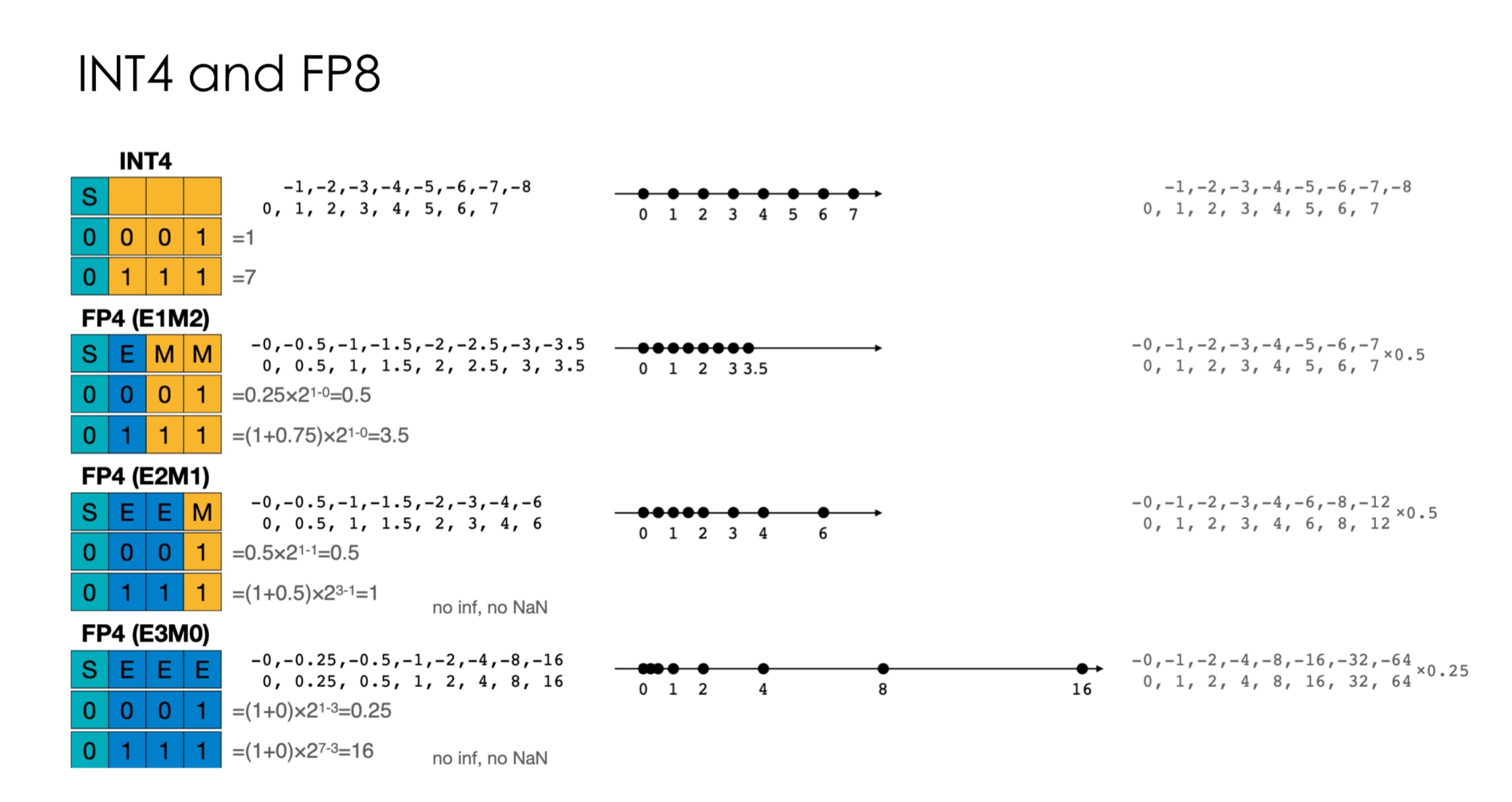
There has been no successful model with these representations, making it a very promising avenue for research.
Alright, with these things in mind, let us come back to quantization. There have been two approaches for quantization
-
K-Means based quantization - widely used, almost all mobile devices have it.
Consider we have a weight matrix that we are trying to quantize. The idea is to cluster close values together into an integer or a lower-precision representation. The number of clusters is chosen based on the chosen requirements - for 2-bit quantization, number of clusters is 4.
To do so, we simply apply K-means. The centroids are stored in a code book whereas the matrix is simply stored in the lowest possible representation to further reduce storage. How do we perform a backward pass on these matrices? The gradients are accumulated based on the classes and are applied to the centroids to fine-tune them. In practice, quantization starts affecting the performance sharply only after a certain threshold. Therefore, quantization becomes a hyper-parameter tuning problem, and we can achieve significantly lower memory consumption. The number of bits used can vary with layers as well!
Try coding a library with variable quantization layers. Shared code books across layers
How is the run-time affected? The computations are still FP arithmetic. There is an added computation cost for weight compression/decompression and code book lookup. K-means has been quite effective with convolution networks.
-
Linear quantization - The idea is to determine a linear mapping of integers to real numbers. It can be seen as a linear optimization problem.
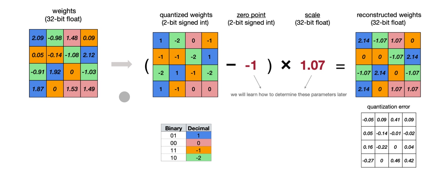
So, we need to determine zero-point and scale parameters. These parameters are often also publicly shared on platforms such as HuggingFace. The parameters can be chosen for the whole model or for each layer based on our performance tradeoff appetite. For many popular models like Llama, the quantization is done tensor-wise.
The parameters can easily be determined as follows
\[\begin{align*} S &= \frac{r_{max} - r_{min}}{q_{max} - q_{min}} \\ Z &= \text{round}(q_{min} - \frac{r_{min}}{S}) \end{align*}\]The bit-width \(n\) determines \(q_{min} = -2^{n -1}\) and \(q_{max} = 2^{n - 1} - 1\).
Suppose we apply linear quantization to
\[\begin{align*} Y &= WX \\ S_Y(q_Y - Z_Y) &= S_W(q_W - Z_W)S_X(q_X - Z_X) \\ Q_Y = \frac{S_W S_X}{S_Y} \left( q_W q_X - Z_W q_X - \underset{Z_X q_W + Z_W Z_X) + Z_Y}{\text{precomputed for inference}} \right) \end{align*}\]matmul-Empirically, the factor \(\frac{S_W S_X}{S_Y}\) is between 0 and 1. Instead of using floating point multiplications, it is represented as fixed point multiplication and bit shift. Also, empirically \(Z_W\) follows normal distribution and can be approximated as 0. Thus, the heavy lifting operation is \(q_Wq_X\) which is simply integer multiplication.
Therefore, we reduced both storage and computation time (integer arithmetic is much faster and cheaper). This can also be used to reduce FP16 to FP8 rather than integers.
In summary, we have 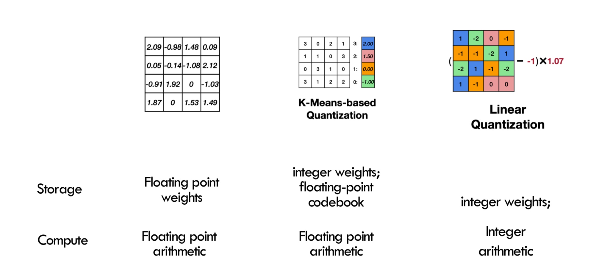
Large Language Models on Cloud and Edge
The first wave of revolution in ML systems was sparked by Big Data in 2010s (competitions like Netflix recommendation price), which resulted in systems such as XGBoost, Spark and GraphLab. Then in mid 2010s, deep-learning started gaining traction, and TensorFlow, TVM and Torch were created. Now, we’re in the third revolution with Generative AI. ML Systems is playing a much bigger role.
The challenges involved are -
-
Memory - Llama-70B consumes 320GB VRAM just to store parameters in FP32
-
Compute - The post-Moore era brings great demand for diverse specialized compute, system support becomes bottleneck
The design of systems depends on the paradigm that the industry is moving towards. Currently, we have cloud based models with a client-server architectures. This is how computers initially started before the age of personal computers. So, would we move towards personal AI in consumer devices?
There are many engineering challenges involved in this. As we covered previously, there are specialized libraries and systems for each backend involving manually created optimizations. The area is very labor intensive with huge market-opportunities.
Our approach to this has been in terms of composable optimizations to rewrite kernel codes. Furthermore, we added techniques such as parameter sharding, memory planning, operator fusion, etc to add to these optimizations. What have we learned from this journey?
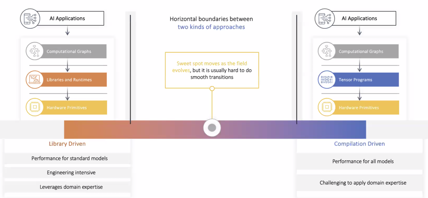
There are four abstractions we use
-
Computational Graphs - Graph and its extensions enable higher level program rewriting and optimization
-
Tensor Programs - These abstractions focus on loop and layout transformation for fused operators
-
Libraries and Runtimes - Optimizing libraries are built by vendors and engineers to accelerate key operators of interests
-
Hardware Primitives - The hardware builders exposes novel primitives to provide native hardware acceleration
It has not been about a silver bullet system but continuous improvement and innovations. ML Engineering is going hand-in-hand with ML modeling.
The developers of TVM are expanding it to TVMUnity to bring the compiler flow to the user. As we’ve studied, IRModule is the central abstraction in TVM. Once the user-level code is written in this form, TVM takes care of the hardware backend making it easy to the models on various architectures.
TVM generates an optimized models, and features are continuously added with data to make it better over time.
TVM Unity
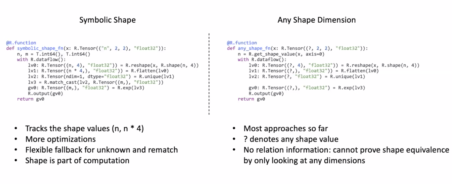
First-class symbolic shape support
Traditional models like ResNet have some key-characteristics. The compilers are being built under the assumption of these fixed parameters, but with the age of generative AI, these parameters keep changing continuously. TVMUnity leverages symbolic shift to incorporate variable sizes in the model. In essence, traditional compilers are unable to handle dynamic shapes, whereas TVMUnity allows it with symbolic support.
Knowing the dependencies between different variable parameters allows for better optimizations during runtime - static memory planning for dynamic shapes
Composable Tensor Optimization
In the early ages, we had scalar computing. Then came the age of vector computing with SIMD. Now, NVIDIA has TensorCore and TPUs became a thing for tensor computing. How do we leverage these hardware developments in our programs? We want both loop based optimization and tensor-based programs.
The first step is to isolate the internal computation tensorized computation from external loops to create a Block.
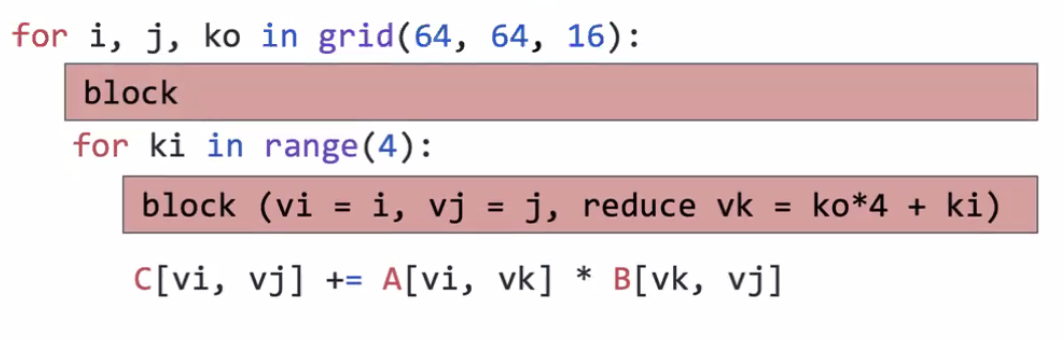
With this, TVMUnity does Imperative Schedule Transformation to search different variants of programs by changing blocks to create an optimized IR.
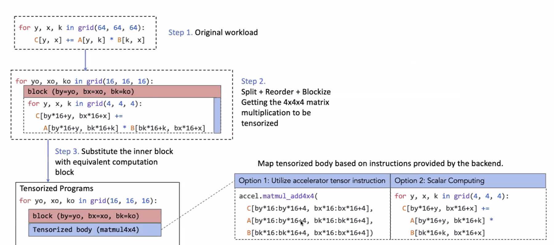
By providing this interface to the user, where the user can mention the parameters involved, TVMUnity can perform tensorization along with graph-optimization problem.
Bringing compilation and Libraries Together
We have seen this tradeoff with compilers and libraries.
TVMUnity provides interfaces like Relax-BYOC to offload the computational load to libraries such as TensoIR to leverage the library-optimized kernels. The native compilation works on top of the library offloading to increase the performance even more.
By adding this flexibility, the compiler can update (live with library updates) to squeeze the best performance.
Since libraries come out with data layout requirements, the compiler can use this information to optimize the remaining parts of the code.
ML Compilation in Action
How does this architecture help with incremental developments? The users can try new optimizations in coordination with the compiler to scale to newer models.
In language models, the compiler does targeted optimizations such a low-bit quantizations, dynamic shape planning, fusion and hardware aware optimizations, etc. Along with these, it works with KVCache etc to improve the performance.
The MLCEngine is a universal LLM deployment engine being developed to deploy LLMs on any device. The key contribution here is universal. This development also revealed some key insights - iOS devices require custom Metal language kernels, Snapdragon devices require OpenCL - and this project is trying to take care of all of that.
It also helps with structured generation with near zero overhead. This feature would be super useful for agent use cases. Surprisingly, MLCEngine does it with near zero overhead with something known as XGrammar!
They also created WebLLM with the new WebGPU standard to use the local compute to the browser. Yes, it uses your local GPUs and doesn’t send your data to any server! You can use this to build stuff on top of it with the typescript API and a Node package. It is an open source project too!
Let us continue our discussion on Quantization. We discussed about quantization granularity (per-tensor, per-channel, group quantizations).
Per-channel quantization is preferred to tensor quantization in some cases because the channels can have very different ranges, and using a single \(S\) can result in lopsided representations. Even then, some applications can lose too much on performance for per-channel quantization. In these cases, group quantization is useful.
Group quantization is more fine-grained. E.g., per vector. It has more accuracy, less quantization error trading off some of the savings.
Can we do some sort of statistical grouping here?
The sweet-spot that works in practice is a two-level quantization that quantizes hierarchically. Instead of using \(r = S(q - Z)\) we use \(r = \gamma S_q (q = Z)\). \(\gamma\) is a gloating-point coarse grained scale factor, and \(S_Q\) is an integer per-vector scale factor. It can be further generalized into multi-level quantization with scale factors for each levels.
So far, we have done quantization of weights. They are static during inference, and so everything works. What if we want to quantize the activations? The stats change with every input. This problem is solved in two ways:
- Moving average - Observed ranges are smoothed across thousands of training steps
- Calibration dataset - Figure out the range from subset of training set
Mixed Precision
In the previous methods, we have done uniform quantization wherein every weight parameter is quantized to the same number of bits. However, what if we use different precision for different weights? Does this improve the performance a lot? The implementation is however very complicated since we have to deal with different data formats. Also, what formats give the best savings and high performance?
These are hard questions. So we throw ML at the problem. We define a cost function to let a model discover the combination of formats that give the best parameters. It was a good research field, and the accuracy of models improved by 10% or so.
After a while, NVIDIA released a paper (it’s a good read) that became the standard for mixed precision training. The intuition for this approach is as follows. Some layers are more sensitive to dynamic range and precision. For example, softmax and normalization layers have a large range of values. We identify such operations and assign them higher precision.
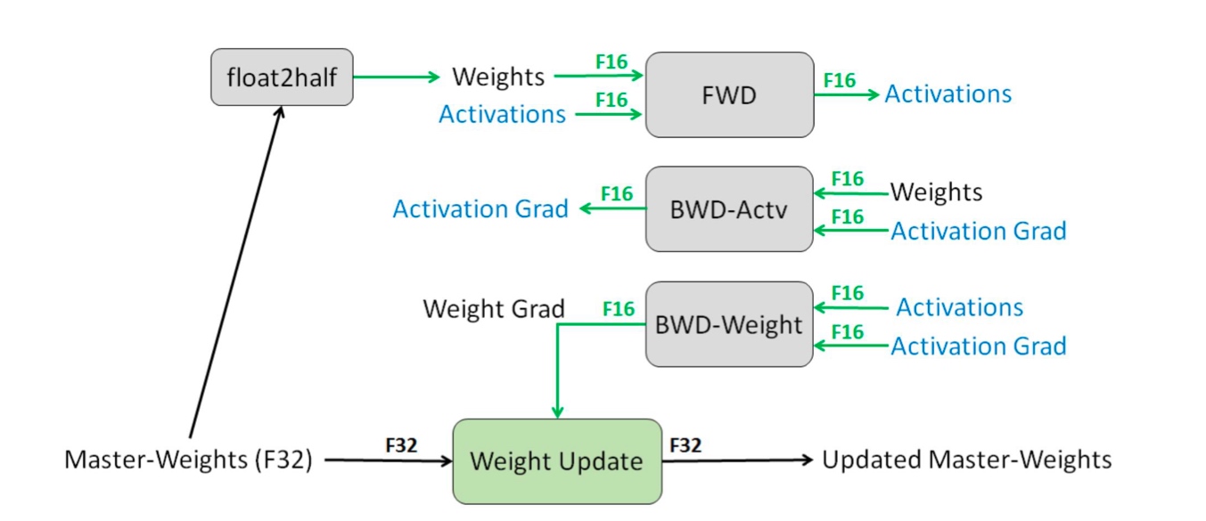
Since Adam calculates two moments and normalizes the gradients, we use FP32 for the weight updates.
Note. Deepseek changed the standard with new precisions.
Let us see how the memory of models changes with this new precision system. Again, for the largest GPT, there are 175B parameters. So it occupies 350G with FP16 for all the weights. The activations occupy 7488G assuming checkpointing at each layer boundary.
So in this system, the master model with FP32 weights occupies 4175 = 700G. The gradients occupy 2175 = 350G. The running copy of the model used for inference is 2175 = 350G. Finally, we need Adam mean and variance (FP32) that is 24*175 = 1400G. The rule of thumb in general is \((4 + 2 + 2 + 4 + 4)N = 16N\) memory for LLMs.
Scaling down ML
Running ML on edge devices is always strongly demanded, and the market is very fragmented. It is easy to build a startup and get acquired in this space. The possible research directions are quantization, pruning, ML energy efficiency, federated ML, etc.
Parallelization
Moore’s law came to an end. However, ML models were scaling 3x every 18 months! Why? Bigger model gives better accuracy. People have also started seeing emergent capabilities in larger models.
So, the models are going to get bigger. Along with this, the memory demand is increasing too. It was back in 2019 when we last fit an entire model in one GPU. Now we require 100s of GPUs just to store the model parameters. The only way out of this is parallelization. Wait! Aren’t GPUs already doing that?
GPUs did data parallelization. We are talking about having multiple GPUs and using them together. All the things we considered so far assumed the entire model is on one GPU. Now, we need to distribute the model training. We just seem to be creating problems for ourselves…
Intuitively there are multiple ways we can go about this
- Parallelize along the layers (cutting through depth)
- Parallelize each layer (cutting through breadth) - this one is rather complicated with more data traveling between clusters.
Apart from these considerations, a GPU cluster also has its own constraints. There are different latency communication channels (kind of like memory hierarchy).
Let us look at the problem from a computational lens. A model involves parameters, weight updates, model spec and the data.
- Computing - The forward pass and backward pass require compute
- Memory - The data and parameters require memory. Between these, we require communication (typically done with interconnects or network, e.g., NVLink) which is the main bottleneck in this whole setup. How do we communicate parameters and activations?
In data parallelism, we partition the data across GPUs and give each GPU a copy of the parameters and gradients. Then, we need to synchronize the updates together across the GPUs before the next iteration.
In model parallelism, we partition the model across GPUs and use the data to update parts of the model. This method is more complicated. Let us delve deeper.
How do we partition a computation graph on a device cluster?
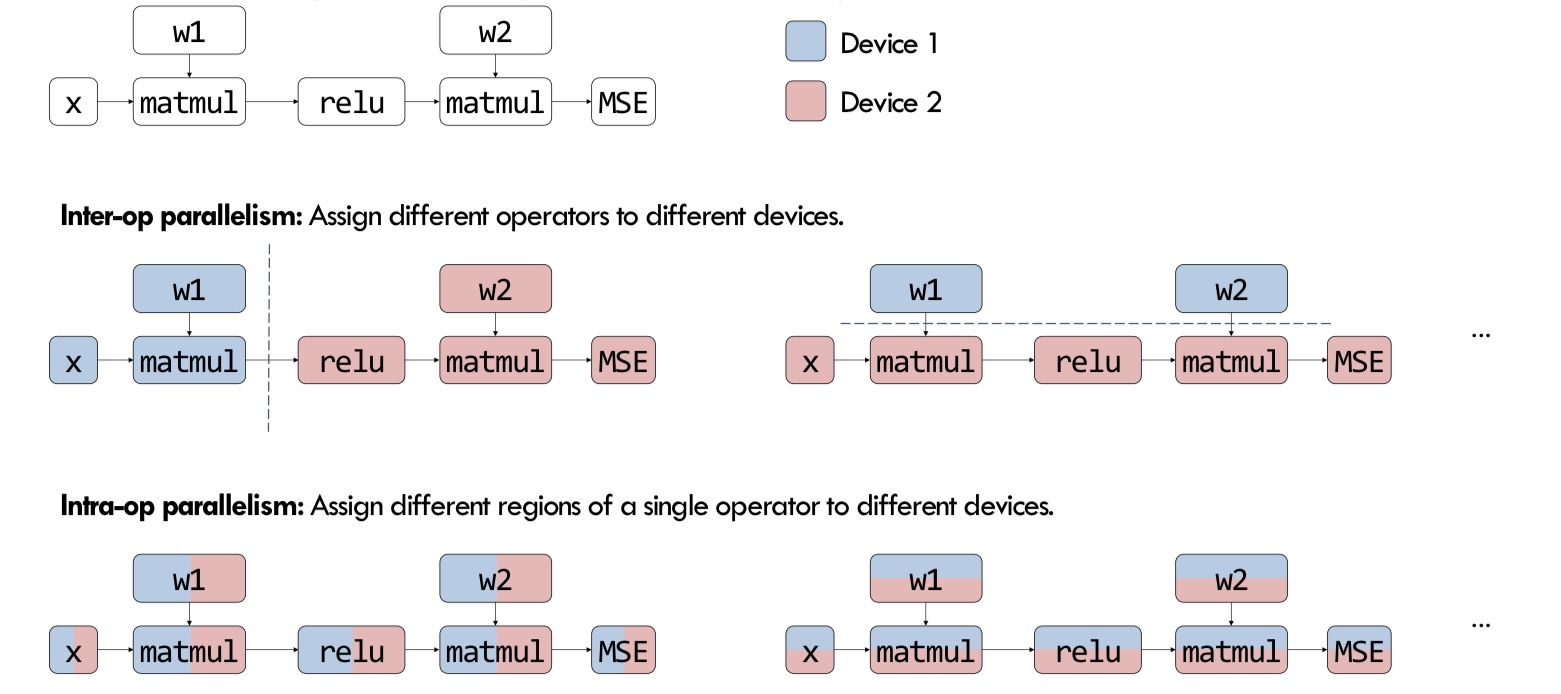
There are more strategies that consider hybrid variants - some parts of the model are inter-op, intra-op and some parameters are replicated across devices.
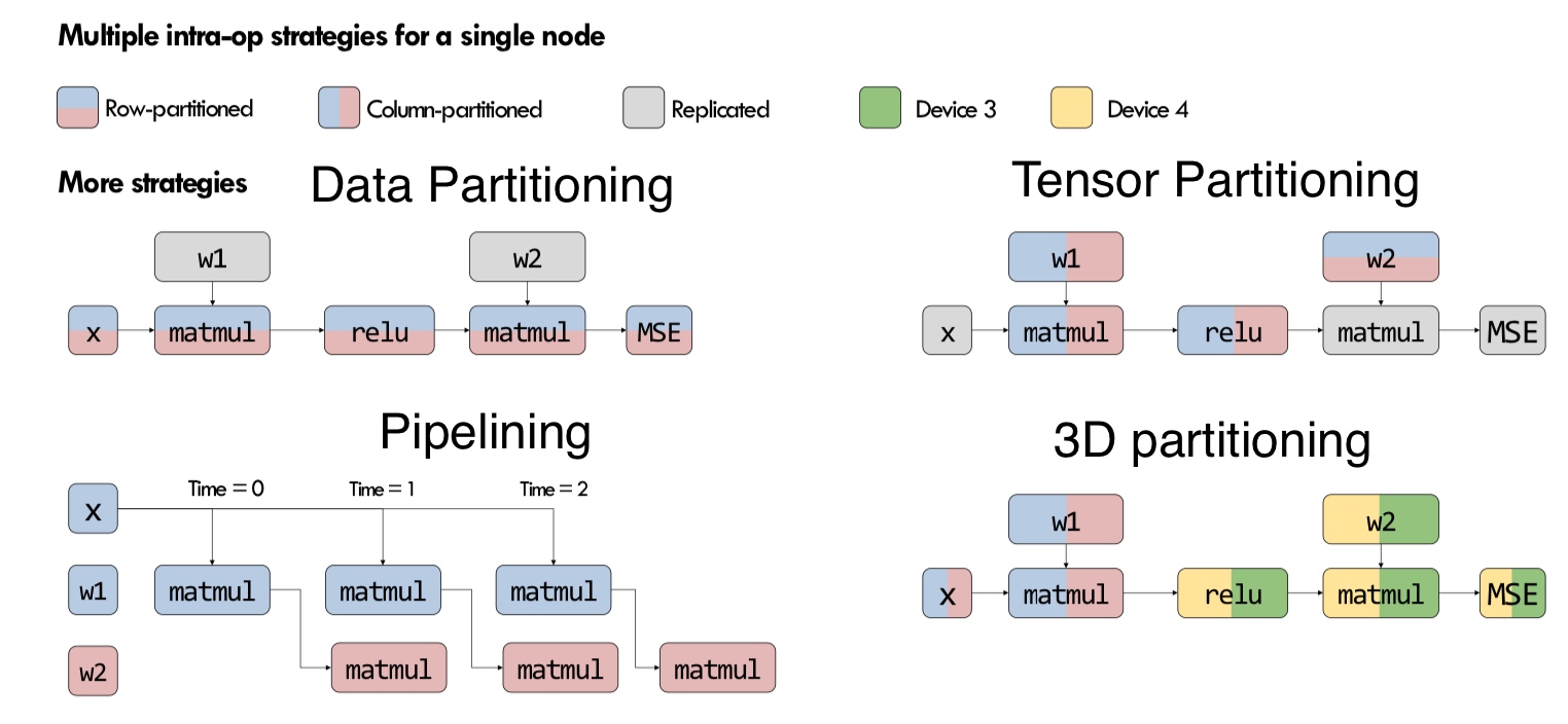
These are the standard techniques being used for the models today.
Let us delve deeper into these. 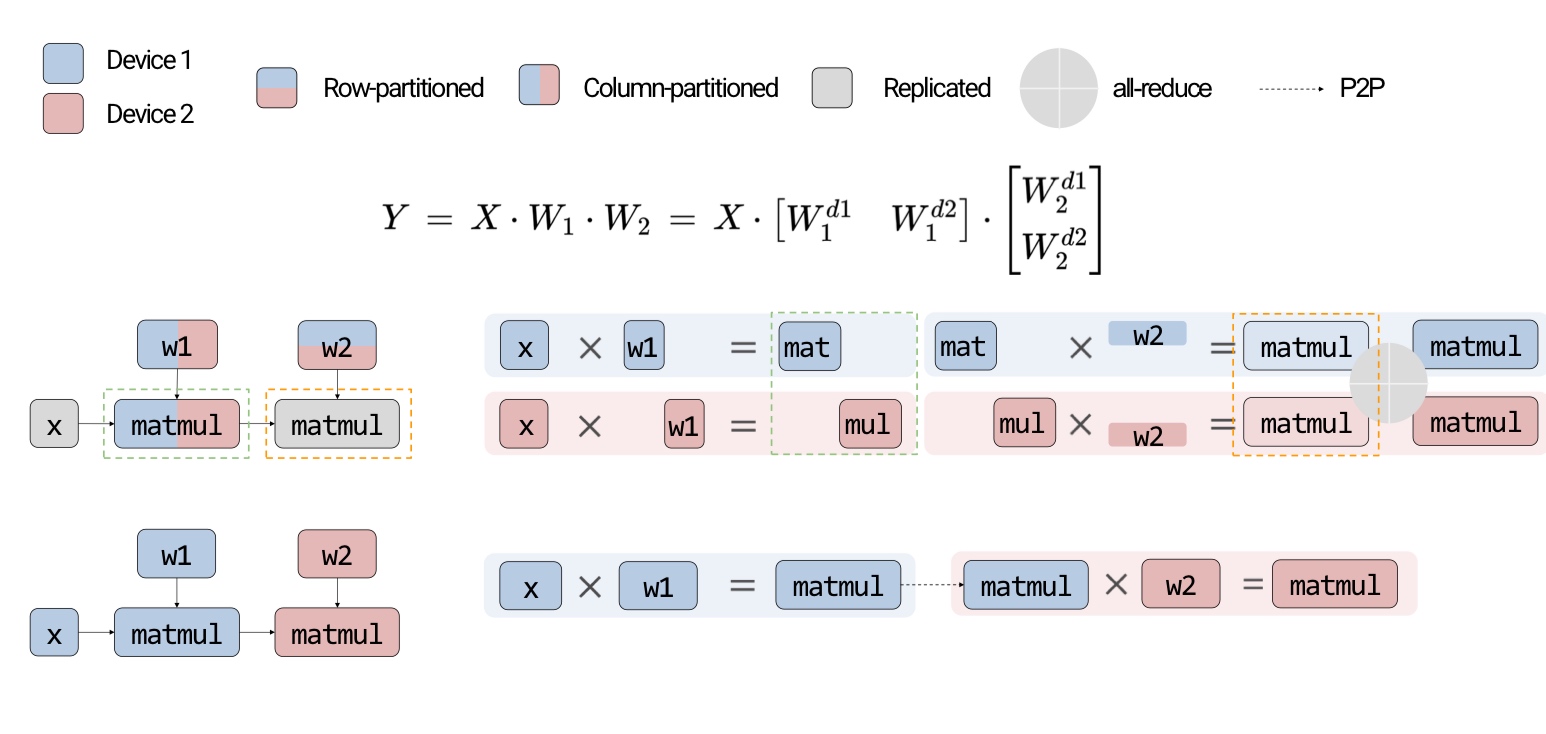 In the above example, intra-op is similar to what we discussed before for matmul on GPUs - each GPU computes a partial sum. Surprisingly, we can show mathematically that this is the best we can do with inter-op.
What are the pros and cons?
- Inter-op parallelism requires point-to-point communication but results in devices being idle.
- Intra-op parallelism keeps the devices busy but requires collective communication.
The all-reduce operation is computationally intensive.
Since intra-op requires more communication, this is an important aspect to consider. On the other hand, inter-op results in hardware bubble wherein some of the GPUs are idle (can be prevented to some extent with pipelining).
In summary, inter-op parallelism requires point to point communication but results in idle devices. The devices are busy in intra-op parallelism but requires collective communication.
A note on terminology Previously, the literature used to talk about data and model parallelism. Data parallelism is general and precise but the term “model parallelism” is vague. That is why, we stick to the terms inter-op and intra-op parallelism which rely on the pillars of computational graph and device cluster. Furthermore, we are mainly discussing about model parallelism because of the regime in which models do not fit on a single GPU anymore.
With that, let us formulate our goal - “What is the most efficient way to execute a graph using combinations of inter-op and intra-op parallelism subject to memory and communication constraints?”
Let us equip ourselves with a metric to quantify this goal. Previously we had, Arithmetic Intensity. Now, we consider Model FLOPs Utilization (MFU)
\[MFU = \#FLOPs/t/\text{peak FLOPs}\]Where #FLOPs is the total FLOPs in the ML program, and \(t\) is the time required to finish the program. The goal is to maximize this quantity.
Why don’t we achieve the peak FLOPs? The Peak FLOPs values are typically achieved by matrix multiplications but a neural network model like a transformer involves many layer operations (memory bounded) that lower the performance. Moreover, we have seen how optimization can greatly reduce the time of execution and increase the operations within the same time. Unoptimized code can lower the value further. Adding to these communication like we have discussed before can reduce the quantity a lot too. Finally, all these parameters also depend on the precision, code and the GPU type being used.
How do we calculate the MFU?
- Count the number of operations (FLOPs) considering the shape of the data in the model. For example, we have seen the formula \(2mnp\) for
matmul. - Run the model for one forward and backward pass on the GPU to get benchmark for the running time \(t\)
- Check the GPU spec, type of cores, and their peak FLOPs
- Calculate the MFU
What is the history of these numbers?
- The best ML system on V100 a couple years ago got 40-50% MFU - only half the peak utilization! The peak FLOPs on V100 is 112 TFLOPs, so we were only able to use 50-60 FLOPs
- With A100, we were still in the same range until FlashAttention came up, which took the MFU value to 60%! A100 has 312 FLOPs, so we are using ~160FLOPs at this stage!
- With H100, we are able to use only 30-50% depending on the model size (Larger
matmulis better for MFU over smaller). Why did it decrease? The peak value of H100 is very high (990 TFLOPs), and our software did not catch up to this. Remember that communication also plays an important role - This year, with B100 the peak FLOPs is 1.8 PFLOPs!
Besides MFU, we also define Hardware FLOPs Utilization (HFU). This quantity is to consider operations that do not contribute to the model For example, we can treat gradient checkpointing as 2 forward passes and 1 backward pass (each backward pass can be approximated as 2 forward passes due to gradient updates)
Collective Communication
In Machine Learning systems, there are usually two types of connections
- Point-to-point communication - Comprises of a sender and a receiver. Very simple.
- Collective Communication - It’s a common concept in HPC (high performance computing). There are multiple forms of this
- Broadcast - One worker shares data with all the other workers
- Reduce(-to-one) - All the data among the workers is combined into one rank (one worker). Essentially reverse of broadcast in a way.
- Scatter - The data from one rank is split and each of the splits is scattered across other ranks. That is, every worker gets on part of the data.
- Gather - The reverse operation of Scatter, where different parts of the data are gathered into one rank.
- All-gather - Essentially gather followed by broadcast.
- Reduce-scatter - Essentially reduce followed by scatter.
- All-reduce - Reduce followed by scatter.
Collective communication is more expensive than P2P since it can be thought of as a combination of many P2Ps. However, collective communication has been highly optimized in the past 2 decades (
(x)ccllibraries - NVIDIA hasNCCLthe best, Microsoft hasMCCLand Intel hasOneCCL). The important thing to note is that collective communication is not fault tolerant (if one device fails, then everything fails).
Basics
Let us understand some more terminology for communication models. There is a terminology called as \(\alpha\beta\) model that talks about latency and bandwidth. For example, if the model is \(\alpha + n \beta\) then \(\alpha\) refers to the latency and \(\beta = 1/B\) is the reciprocal of bandwidth determined by the hardware. For smaller messages, latency (\(\alpha\)) is the dominant factor, and for larger messages (larger \(n\)), the bandwidth utilization (\(n\beta\)) dominates.
Based on these distinctions, the community works on two mainstream algorithms/implementations
- For smaller messages, an MST based algorithm that emphasizes low latency
- For larger messages, a Ring algorithm to emphasize on bandwidth utilization.
There are over 50+ algorithms in this area and the HPC community even got the 2023 Turing award!
The core principle for lower latency is to minimize the number of rounds needed for communication. For example, consider the Broadcast operation.
- We first split the ranks into half, and send the message to the half without the message
- Then repeat broadcast recursively in each half
Beautiful.
For the core operations, we have the following communication models
- Reduce-to-one - \(\log(p) (\alpha + n \beta + n \gamma)\)
- Scatter and Gather- \(\log(p)\alpha + \frac{p - 1}{p} n\beta\)
- Broadcast - \(\log(p)(\alpha + n \beta)\)
The remaining composite operations can simply use these primitives.
What are the problems with this approach? Since latency is prioritized over bandwidth, some links are idle. Building on the same idea, the core principle for high-bandwidth is to use all links between every two nodes.
The ring algorithm essentially is a logical ring that can be embedded in a physical linear array with worm-hole routing such that the “wrap-around” message does not conflict. Look at the diagram below for clarity -
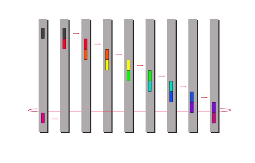 At every instant, all the links are used ensuring full-bandwidth. For example, reduce-scatter can be implemented as consecutive reduce and propagate ring passes.
For this regime of communication, the core primitives of communication are
- Reduce-scatter
- Scatter
- Gather
- All-gather and the other operations can be implemented as the composites of these
- Reduce(-to-one) is reduce-scatter followed by gather
- All-reduce is reduce-scatter followed by all-gather
- Broadcast is scatter followed by all-gather.
So, how does this all come back to ML? ML systems are usually composed of large data communications. Inter-op systems always result in P2P communications and intra-op result in collective communication.

The key point to note is that communication always happens between nodes that are partitioned differently. Remember that with tensors there are more dimensions, and the above diagram is a simplified version. Just to summarize all ideas and the motivations behind our discussions, let us go through this again.
Data Parallelism
Data parallelism was first suggested by Dean et. al. In DistBelief based on a Parameter server. This method was mainly based on sharding the data through batches. Then, this paradigm evolved, and integrated into PyTorch as DDP.
When using data parallelism, there are two solutions to update the model parameters (assuming the models can fit inside one GPU worker)
Parameter server
As proposed in the original DistBelief paper, the parameter server is to help with gradient descent (not stochastic). The gradients are accumulated across the workers (have to wait for all workers) and are used to update the parameters. These parameters have to be replicated across all workers for further forward computations (server bottleneck). The compute to communication ratio for this is 1:10 in 2021.
This approach can be improved to some extent by using a distributed parameter server (sharded KV stores). This ensures a redundancy across different PS shards. The savings essentially comes from using AllReduce - no server bottleneck and faster gradient sharing by workers. When the parameter server nodes are same as the worker nodes in the previous setup, the configuration simplifies a lot more. The operations then become Reduce-scatter followed by Allgather.
Even then, one slow worker can slow down the whole system.
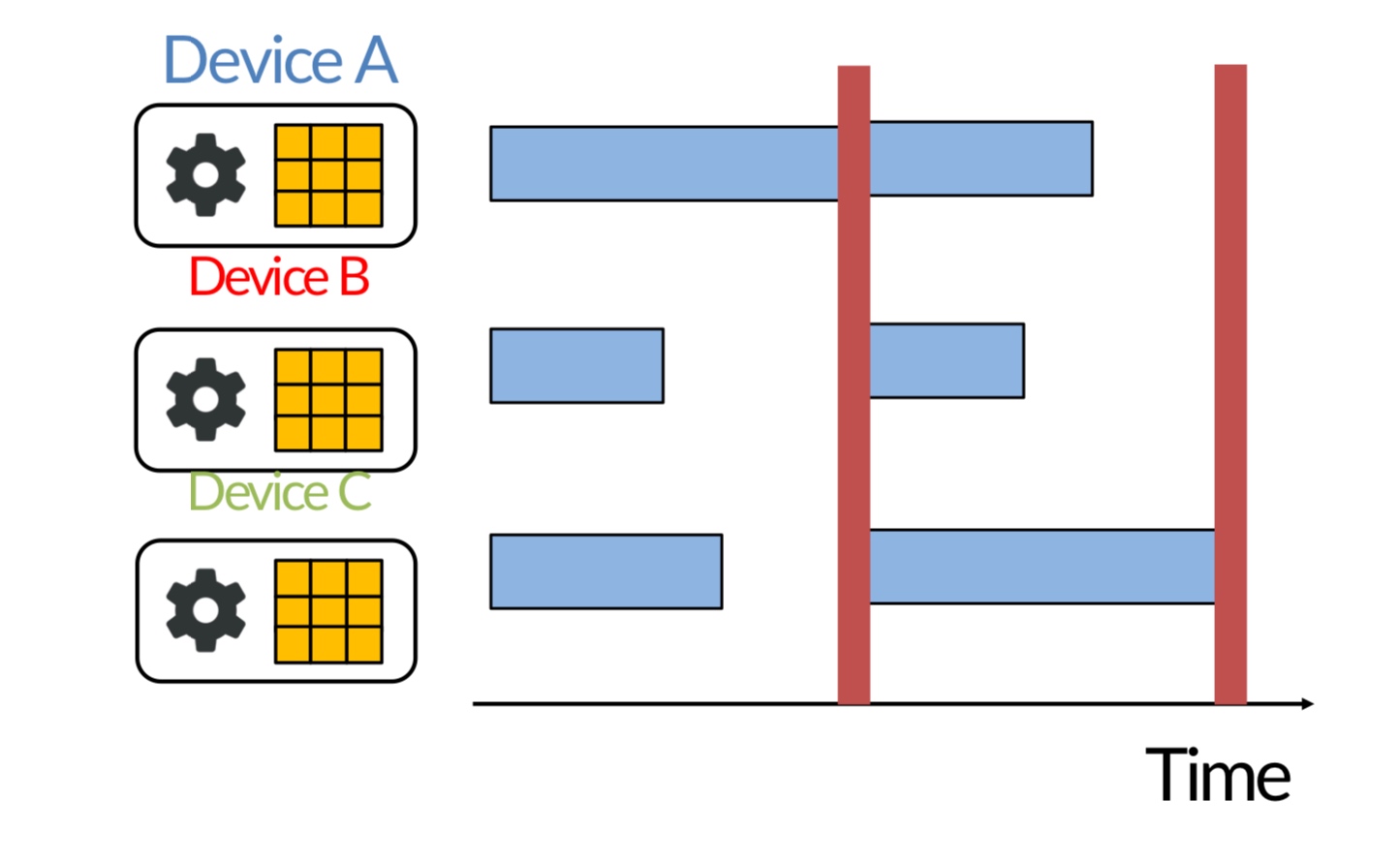 The problem is that we have been waiting for all workers to update the parameters. However, machine learning systems are error-tolerant to some extent. Deviating from the gradient can still lead to the same performance (similar to why stochastic gradient descent works).
So adopting a form of asynchronous communication wherein the parameters are updated every time a worker finished the computation. We can set a staleness threshold to discard very old messages for improved performance. It turns out that the training stability is heavily dependent on this parameter. There were a lot of theorems for this line of work too!
All-Reduce
DDP is a form of Allreduce type of data parallelism. Allreduce was initially implemented in Horovod (was designed by Uber!). It was further optimized by NVIDIA in NCCL. It was then adopted in PyTorch as DDP.
Also, Allreduce is less fault-tolerant than parameter server! However, this paradigm is more popular since ML systems are somewhat robust to noisy updates. Allreduce does not have consistency mechanisms too!
It became popular due to its simplicity as also because of the release of NVLink - more helpful for Allreduce.
Model Parallelism
As we’ve discussed model parallelism is usually paired with data parallelism (once models stopped fitting in one worker). There are two kinds of sharding - inter-op and intra-op.
Inter-operator Parallelism
Inter-op parallelism usually has smaller communication requirements since only outputs at stage boundaries have to be transferred. However, unless pipelining, there are many hardware bubbles. Without pipelining, we have a bubble percentage of \((D - 1)/D\) and with pipelining we have \((D - 1)/(D - 1 + N)\) where \(D\) is the number of devices and \(N\) is the number of inputs.
Note that we are ignoring the computation models for starting GPU kernels and other overheads for simpler models.
However, this is mainly for inference. For doing backward pass, the devices need to be executed in reverse! Pipelining won’t do. So, how do we reduce the bubbles for training?
-
Device Placement - Slice the branches of a neural network into multiple stages so they can be calculated concurrently.
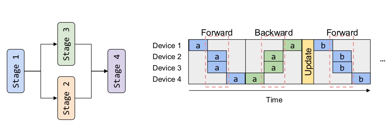 This only works for models with branches such as the Inception model. Contrastive models also include branches and can be used. Other convolutional networks and transformers cannot be used with this.
 - Synchronous Pipeline Parallel Schedule - Modify pipeline schedule to improve efficiency, but keep the computation and convergence semantics exactly the same as if training with a single device. The advantage is that the training process is exactly the same. However, pipeline bubbles are always present and reducing pipeline bubbles typically requires splitting inputs into smaller components, and smaller inputs may not use the hardware to the fullest extent.
- GPipe (Google) - Partition the input batch into multiple “micro-batches”, and accumulate the gradients of the micro-batches.
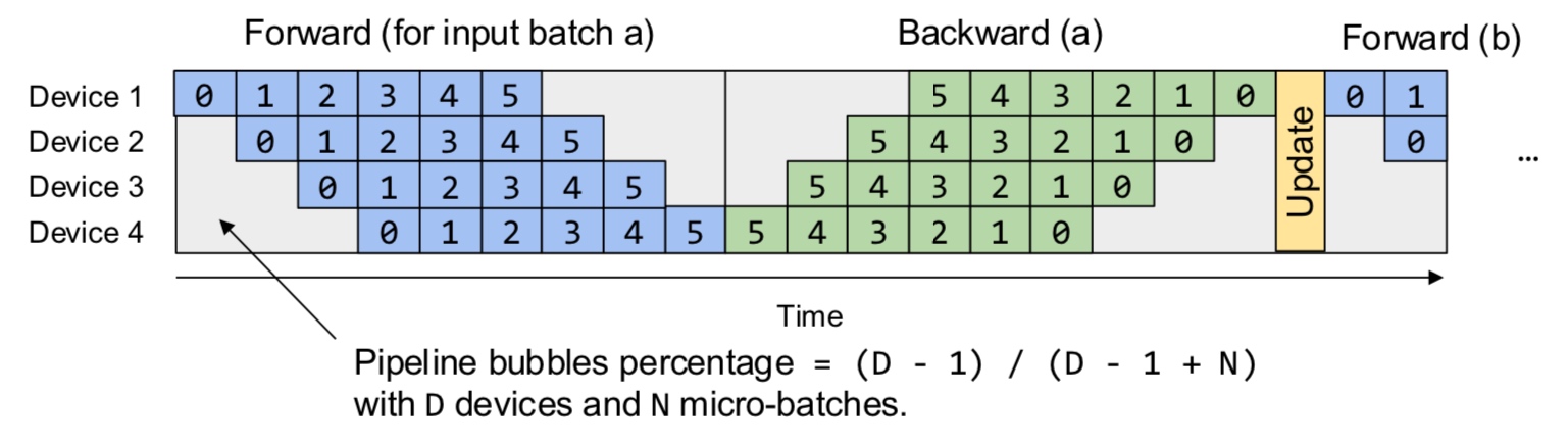 The size of the microbatch has to be chosen so that each device is utilized to the full extent to maintain high arithmetic intensity. This choice is hard to consider. Due to the structure of GPipe, the memory usage of each device increases linearly to a peak and reduces. Each device has to store the outputs from the micro-batches until the backpropagation is called.
 - 1F1B - To prevent this memory peak, the 1 forward, 1 backward schedule was introduced. The idea is to perform backward pass as early as possible.
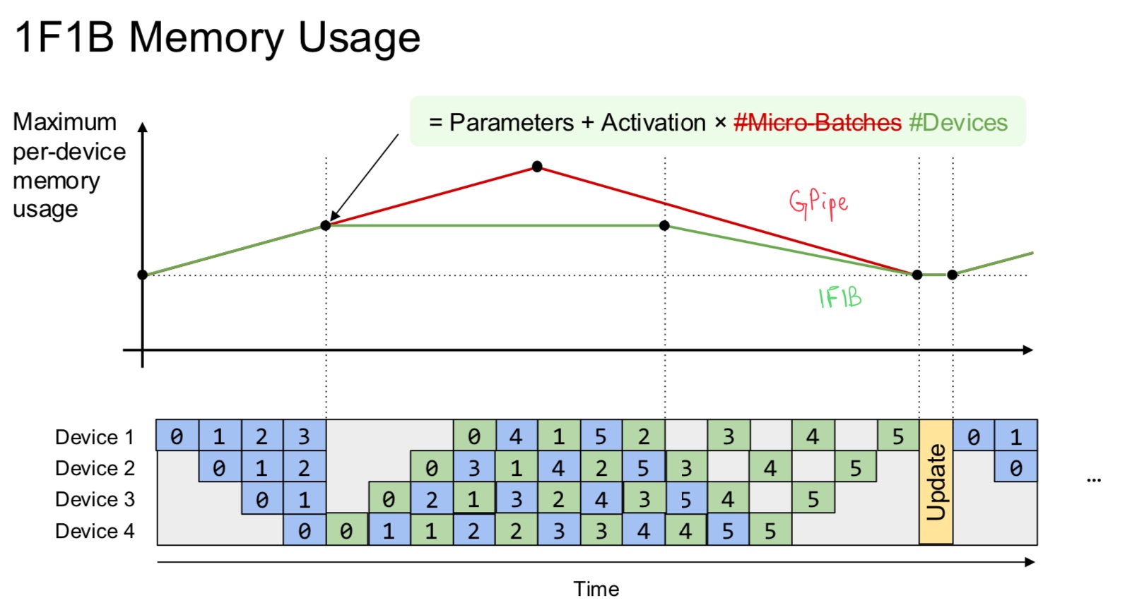 It maintains the same latency as GPipe but with a lower memory usage. (Exam)
 - Interleaved 1F1B - The previous idea can be optimized further to slice the neural network into more fine-grained stages and assign multiple stages to reduce pipeline bubbles.
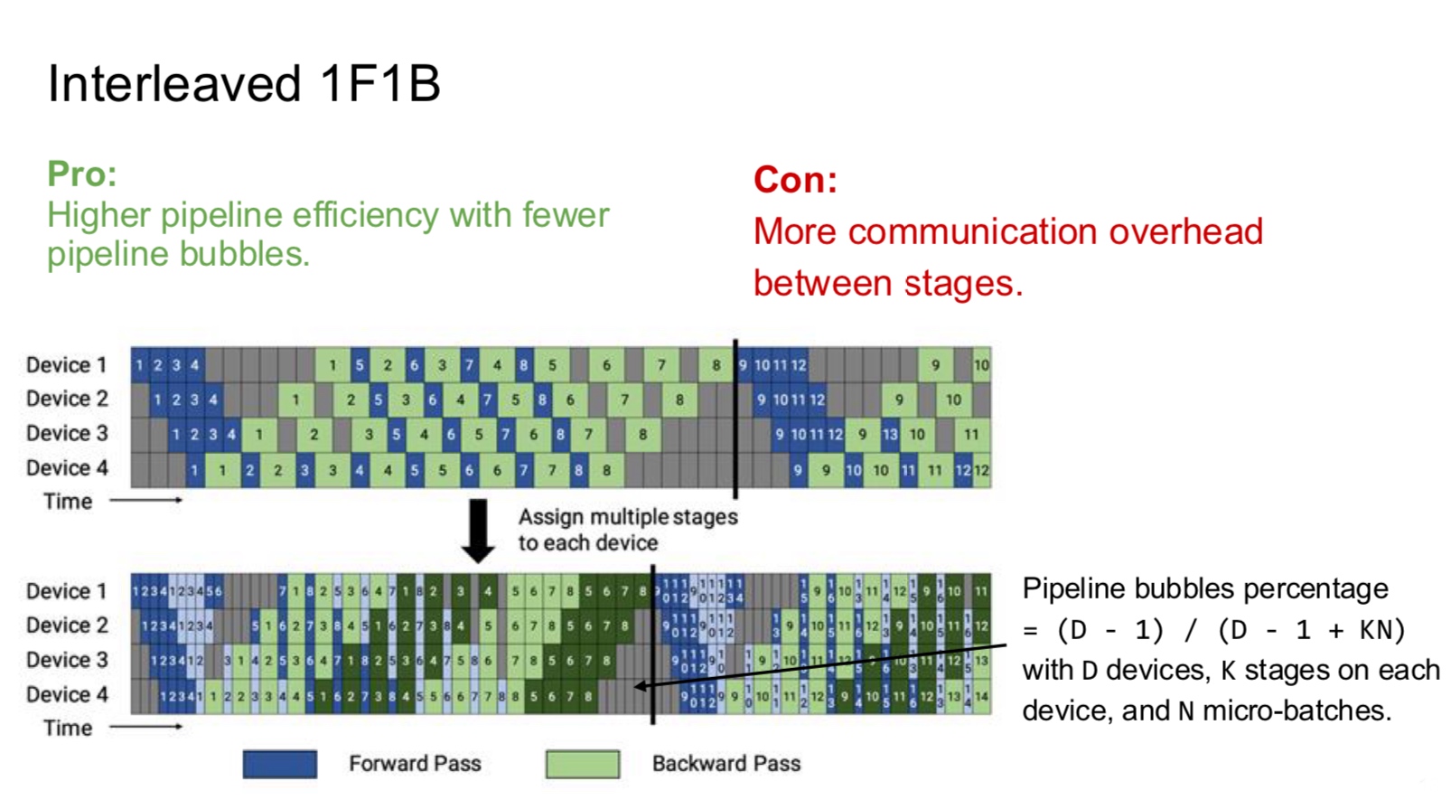 This is super hard to debug.
 -
TeraPipe - This method was mainly suggested for autoregressive models. The key idea is that the computation of an input token only depends on previous tokens but not the future tokens. The bubbles are reduced by pipelining with a sequence.
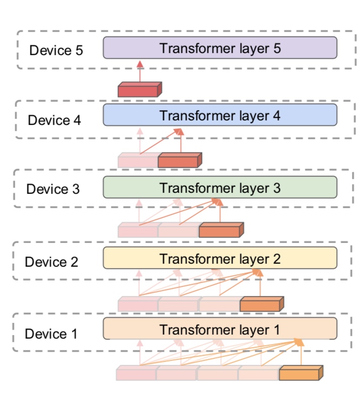
- Chimera - Store bi-directional stages and combine bidirectional pipeline to further reduce bubbles. Deepseek used this! Optimized 1F1B schedule
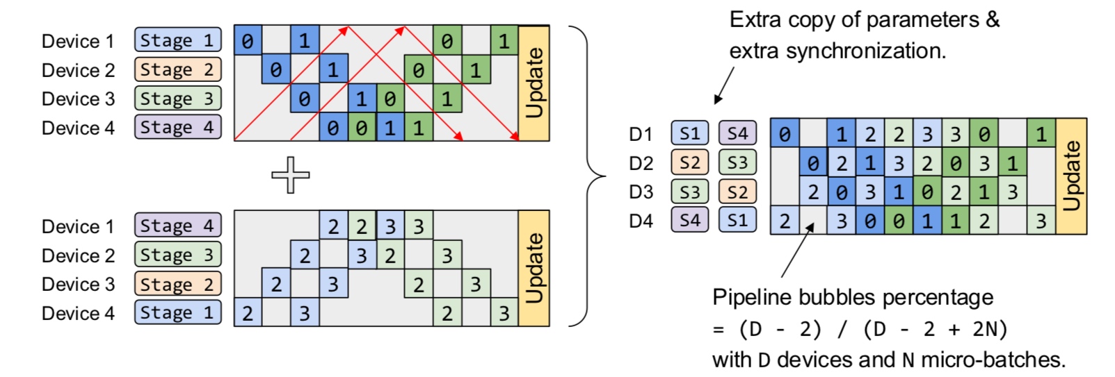 The only issue is that the model parameters have to be stored twice. But if you use a model with half the number of parameters, then you’re good!
- GPipe (Google) - Partition the input batch into multiple “micro-batches”, and accumulate the gradients of the micro-batches.
- Asynchronous pipeline schedules - The idea is to start the next round of forward pass before the backward pass finishes. It breaks the synchronous training semantics, and training involves stalled gradients. The algorithms may have to store multiple versions of model weights for consistency.
-
AMPNet - Each device performs forward pass whenever free and updates the weights after every backward pass. It does not generalize well to larger datasets.
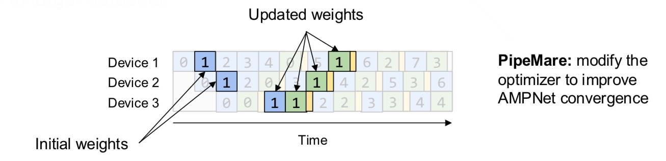
- Pipedream - Enforce the same version of weight for a single input batch by storing multiple weight versions. Has a similar accuracy on Image Net with a 5x speed up compared to data parallel.
- Pipedream-2BW - Reduced memory usage by only storing 2 copied and updating the weights less frequently. The weights are always stalled by 1 update. It achieved similar accuracy on larger models like BERT and GPT.
-
Imbalanced pipelines - All these schedules work best when the stages are balanced. However, there can scenarios where the stages do not have equal workloads. There have been works for automatic stage partitioning that try to minimize maximum stage latency and maximize parallelization.
Placeto: RL-based partitioning algorithm - The state is given by the device assignment plan for a computation graph, and the actions are modifying the device assignment of a node. The rewards are latency differences between new and old placements.
In summary, inter-operator parallelism assigns different operators of the computational graph to different devices and executed in a pipelined fashion.
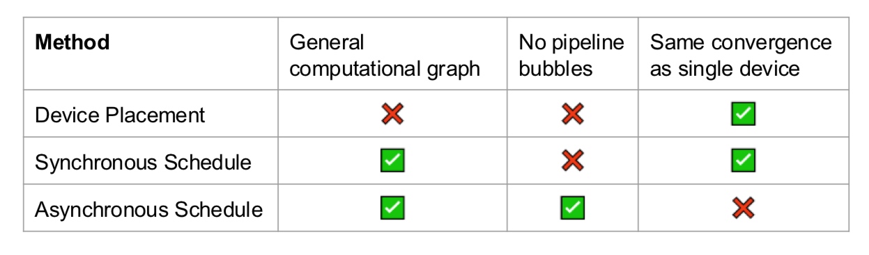
Furthermore, imbalanced stages cause further pipeline bubbles, and RL-based/optimization-based automatic stage partitioning techniques are being explored.
Intra-op parallelism
Let us understand some core ideas to implement techniques in this paradigm.
Suppose we are parallelizing one operator.
- Element-wise operations - The operations involved are typically independent of one another and can be parallelized across devices.
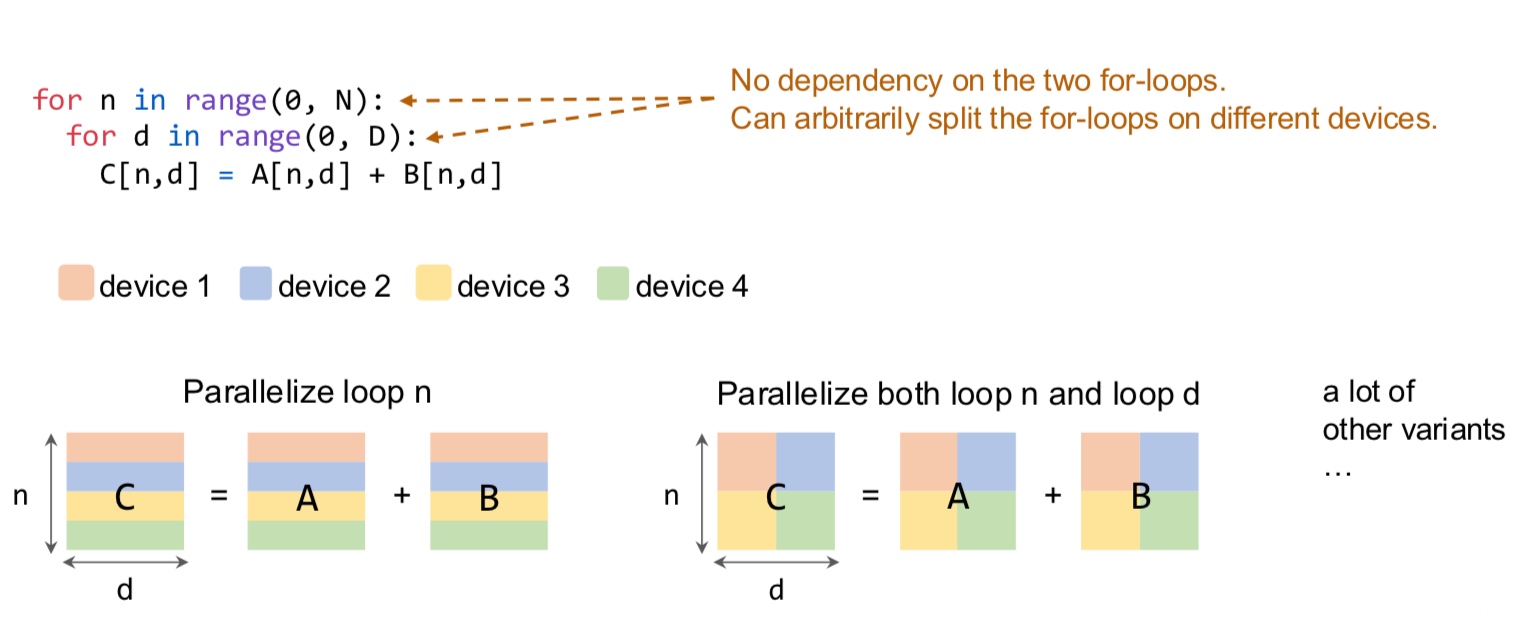 The splitting can be done based on the optimal parameters for the underlying hardware.
 - Matrix multiplication - It is a 3-level nested for-loop. We have the following variations
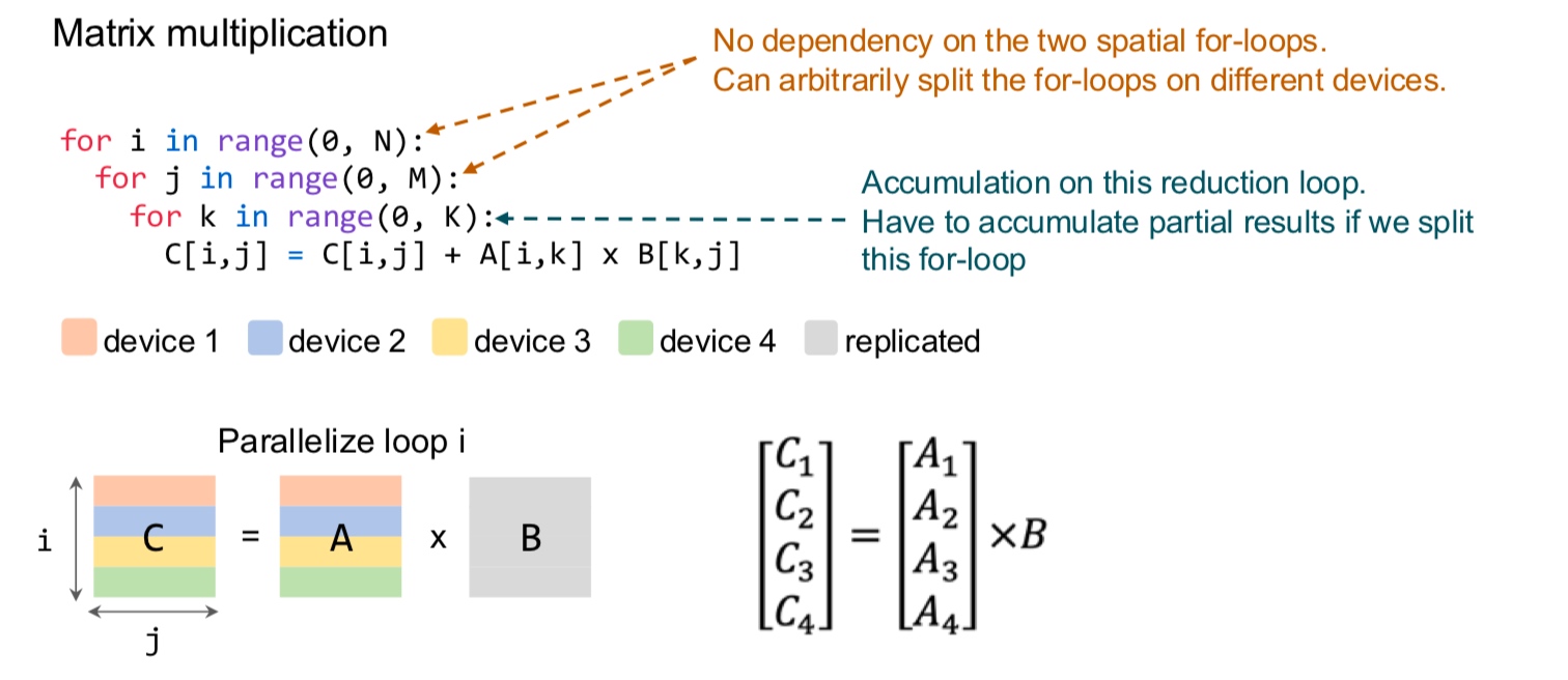
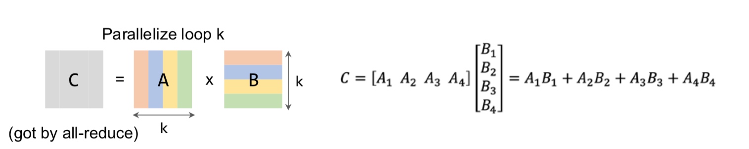
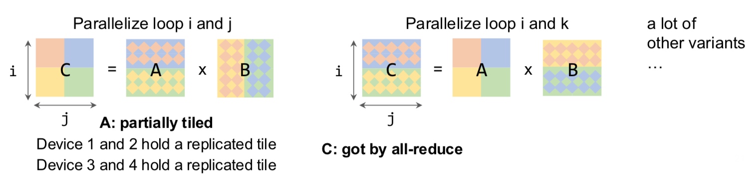
- 2D convolution - It is a 7-level nested for-loop as we’ve seen before.
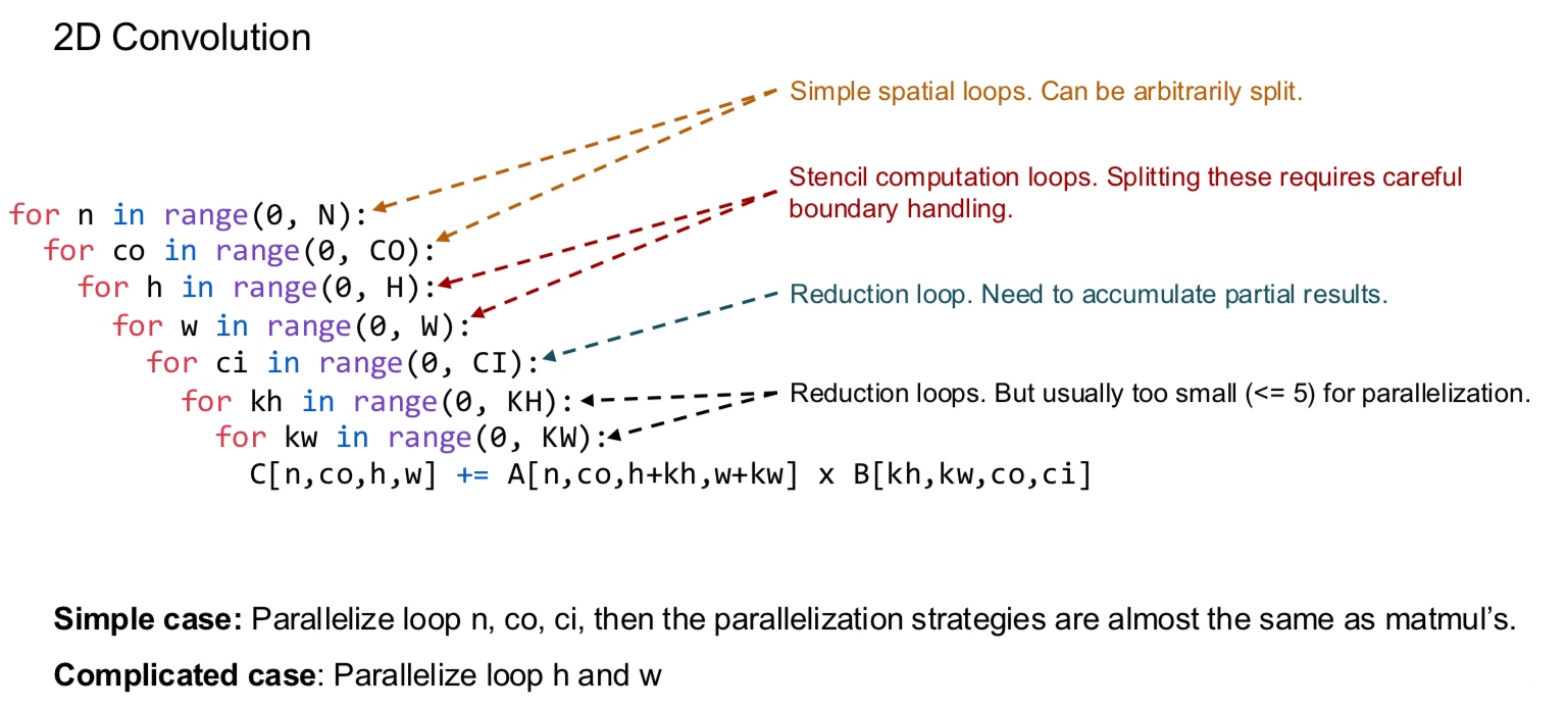
Now, we consider how we parallelize multiple operators together. Note that data parallelism can be seen as a special case of intra-op parallelism. We will consider two main types of matrix multiplication parallelization strategies.
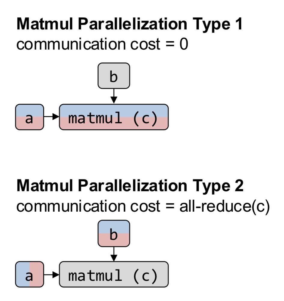
Different parallelization strategies for operators require different partitioning format of the same tensor. For example, with type 1 matrix multiplications, a ReLU operator following matmul would not require any repartitioning. However, in Type 2, we would require an all-gather operation.
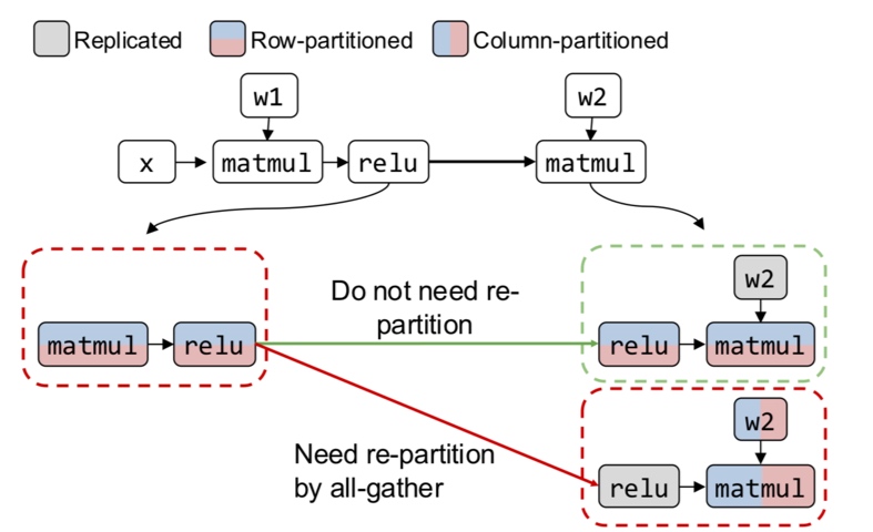
So given these variations, our goal is to minimize the node costs (computation and communication) and the edge costs (repartitioning communication). There have been various solutions using manual design, randomized search, dynamic programming and integer linear programming. We discuss some important projects.
Model-specific strategies
- AlexNet - A convolution layer was split across 2 GPUs. It improved the accuracy by 2%, because the training improved on using 2 GPUs.
-
Megatron-LM - A large language model with 8.3B parameters that outperforms SOTA results! They noted the following - performing Type 2 matmul followed by Type 1 matmul results in only 1 all-reduce operations for both forward and backward passes.
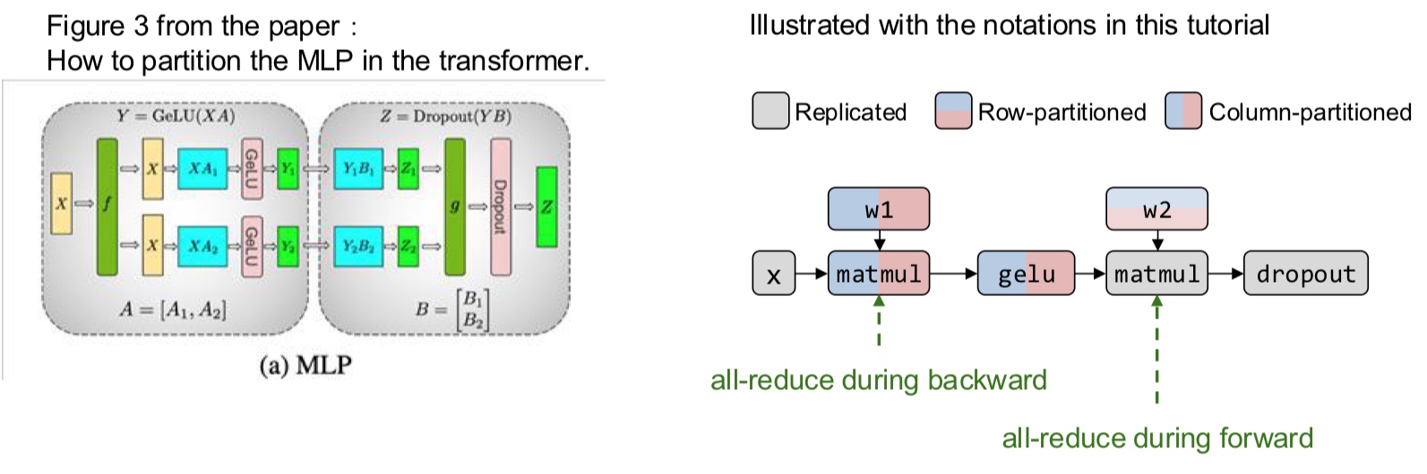
- GShard MoE - A multi-language translation model with 600B parameters that outperforms SOTA.
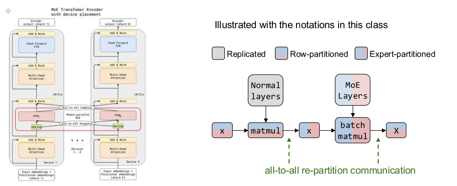 Deepseek used this kind of parallelization, and so they optimized all-to-all operations in their pipeline. These implementations were shared as part of their open-source week event.
Systems for Intra-op parallelism
- ZeRO Optimizer - The authors noticed that data parallelism replicates gradients, optimizer states and model weights on all devices. So, they partitioned gradients, optimizer states and model weights too! Here is a summary -
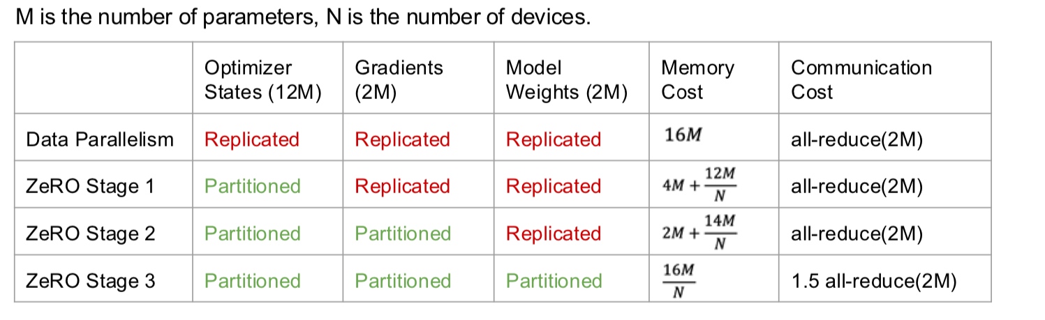 The memory cost in the above table is per device. ZeRO Stage 3 is part of PyTorch through
 FSDP(Fully Sharded Data Parallelism).Recall why the optimizer, gradients and model weights have the mentioned memory costs. Optimizer states are stored in FP32 (factor of 4) and the rest are in FP16 (factor of 2).
Due to the communication and memory costs, everyone prefers Stage 2 over Stage 1 today.
- ZeRO Stage 2 - The operation
all-reduceisreduce-scatterfollowed byall-gather. Using this idea, ZeRO stage 2 does the following.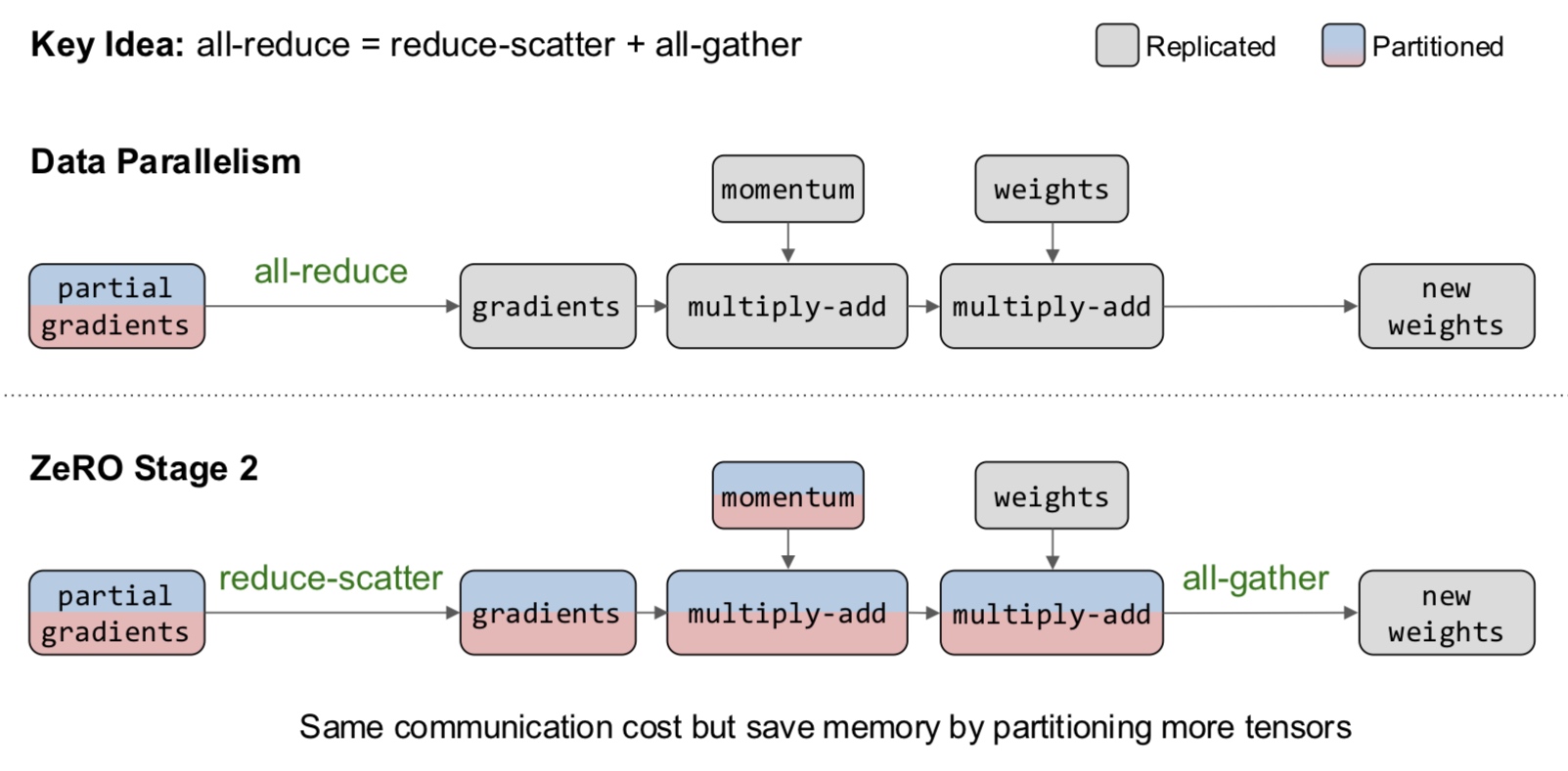 We obtained the same results but with much larger memory savings.
 - ZeRO Stage 3 - Extending this idea, we partition the model across the ranks.
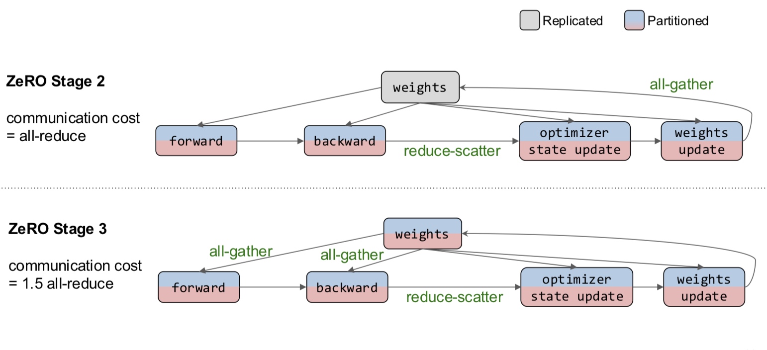 The trade-off between Stage 2 and Stage 3 is memory vs communication cost.
- ZeRO Stage 2 - The operation
- Mesh Tensorflow - The idea is to map tensor dimensions to mesh dimensions for parallelism. A mesh is essentially a matrix of devices.
- GSPMD - Successor for Mesh Tensorflow (a compiler based approach) but generalizes it. The users do not have to partition every tensor, the compiler takes care of automatic partitioning across the code. That is, the annotations are propagated to the whole graph.
- There are more works like Tofu and FlexFlow which we do not cover here.
Now that we have methods for both intra-op and inter-op, how do we combine the both of them? Such kind of a hybrid approach is compulsory to scale the parallelism to clusters that have 1000s of GPUs.
Remember that these can be combined with the approaches we described before for the best outcome.
- System-level memory optimizations - Gradient checkpointing or memory swapping
- ML-level optimizations - Quantization, Sparsification and Low-rank approximation.
Auto-parallelization
The motivation to develop auto-parallelization is very similar to why we designed ML compilers for operator optimization. There are many parallelism models on different model architectures. It is difficult to keep track of which method is the best for a given model and the hardware cluster configuration.
Again, the search space is huge because there are 100-10k operators in a model, 80-200 operator types and number of GPUs in a cluster vary from 10s to 1000s! There have been a multitude of methods for this problem -
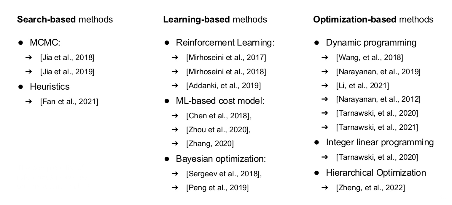
-Search-based methods simply search the best configuration for a given model and cluster. Most companies rely on this technique. It is similar to a brute-force approach.
- Learning-based methods - Uses some sort of learned heuristic to navigate the search space. The most popular work is ColocRL by Mirhoseini et al. That searches the space of inter-op strategies using an ML model to sample candidates and use a policy gradient algorithm to improve the model based on the execution cost. The method was able to obtain strategies that are 20-30% better than an expert-designed assignment. However, the method is not very efficient since it consumes a lot of resources, and RL is not very efficient as well.
-
Optimization-based methods - Search methods but with better optimizations. One good method in this category is Alpa by Zheng et al.. It tries to optimize considering both inter and intra-op parallelism considering the fast and slow connections in the GPU cluster. Intra-op parallelism strategies require communication, so splitting them across ranks with NVLink is a good heuristic. Inter-op can be done across slower communication methods. The method performs the search in a hierarchical manner - inter-op followed by intra-op.
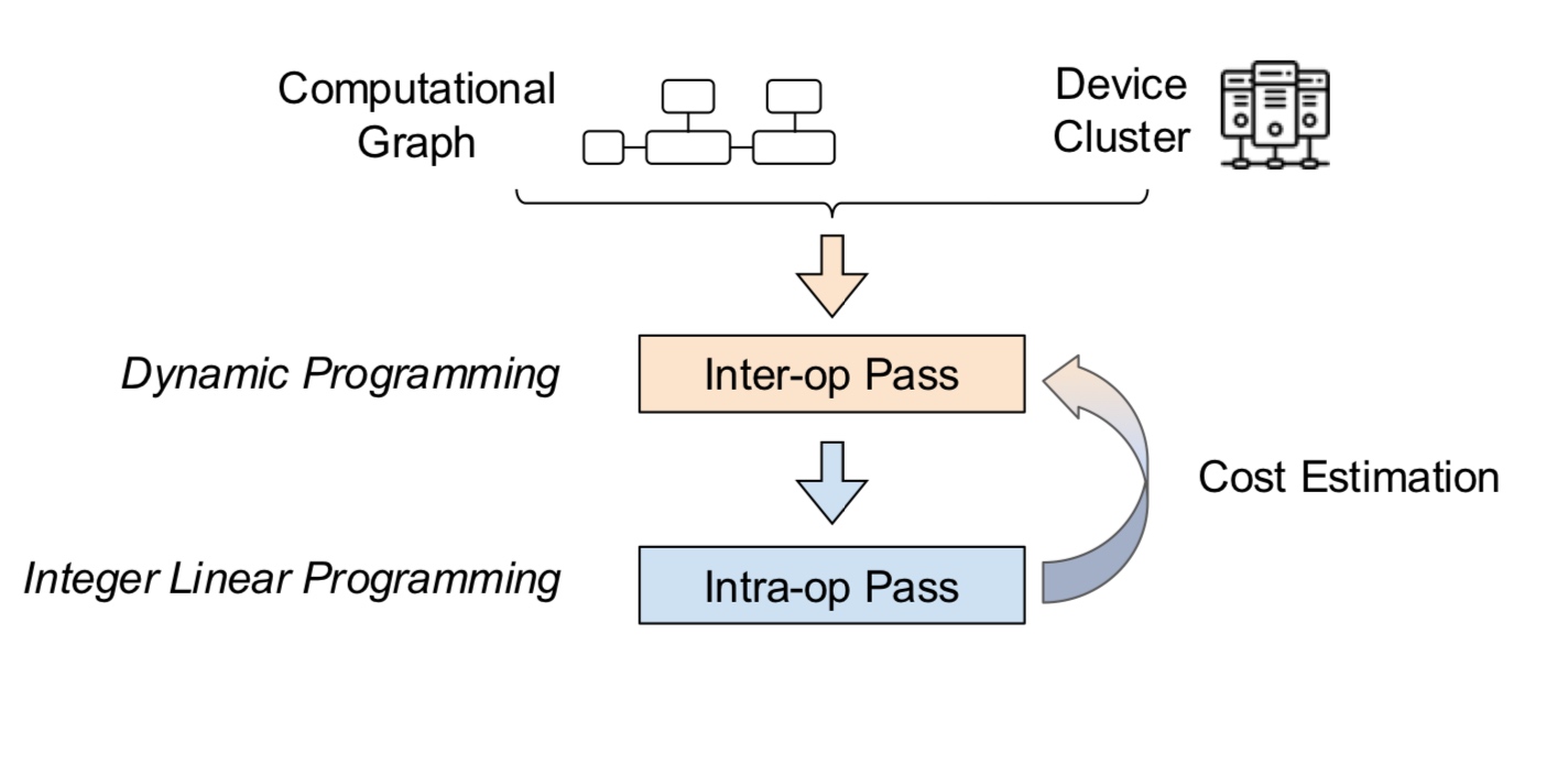
- The inter-op pass, the graph is partitioned into multiple stages, and each stage is assigned different ranks. The states in the dynamic programming algorithm are formed by these choices - partitioning and the sub-mesh assignment. This step also considers the pipeline execution latency, due to different running times of each stages. The running times are given by the intra-op passes, and we have that information. Since dynamic partitioning can introduce imbalances in the pipeline increasing the bubbles, we use dynamic programming with the execution times of each stage to correctly optimize and reach the best strategy. Essentially, the inter-op pass is like the outer loop and we have the information from the inner-loops (intra-op passes) for optimization.
- The intra-op pass parallelizes the operators across sub-meshes and minimizes the communication. For example, consider the following -
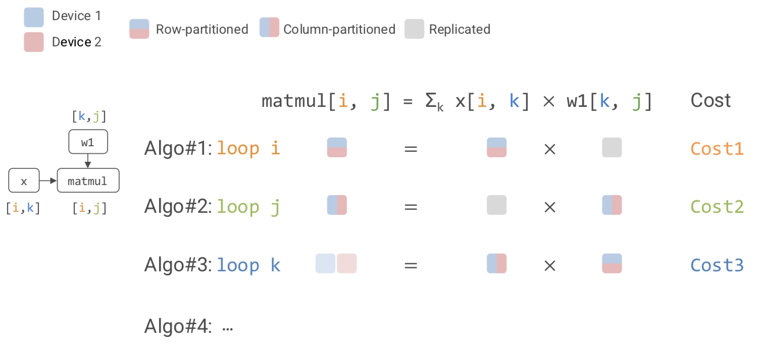
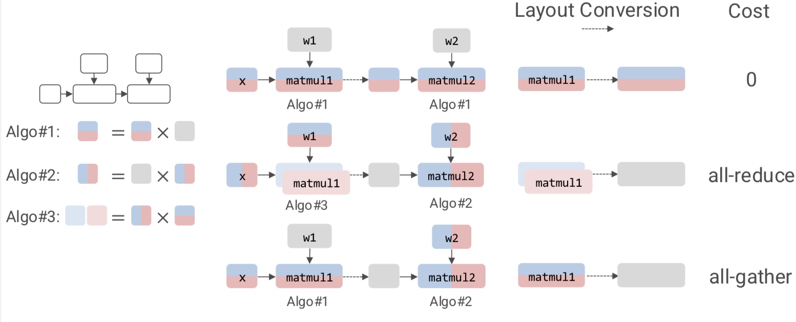
What about the split cost?
Essentially, within each stages, we try to color every node in the stage so that the execution latency of the stage on the assigned mesh is minimized such that the peak memory usage does not cross the memory budget. Note that this problem formulation has node costs (splitting the operator) and edge costs (layout conversions).
With this hierarchical optimization, Alpa is able to
- Match specialized manual systems with GPT
- Outperform the manual baseline for Mixture of Experts by up to 8x
- Generalize to models without manual plans
However, the paper is not popular because the industry has stuck to one type of model (transformers) and the manual expert design for these has been good enough.
In summary, we have
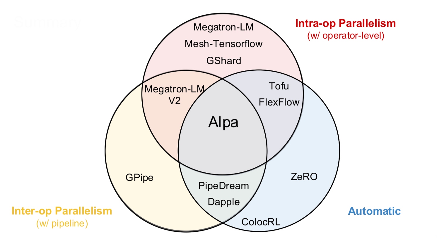
How to choose parallelism then? Transformers have been heavily optimized manually, follow Hao’s ultimate guide below. Otherwise, use the automatic compilers.
We consider the following factors - #GPUs, Model size, JCT (Job completion time), communication bandwidth, etc.
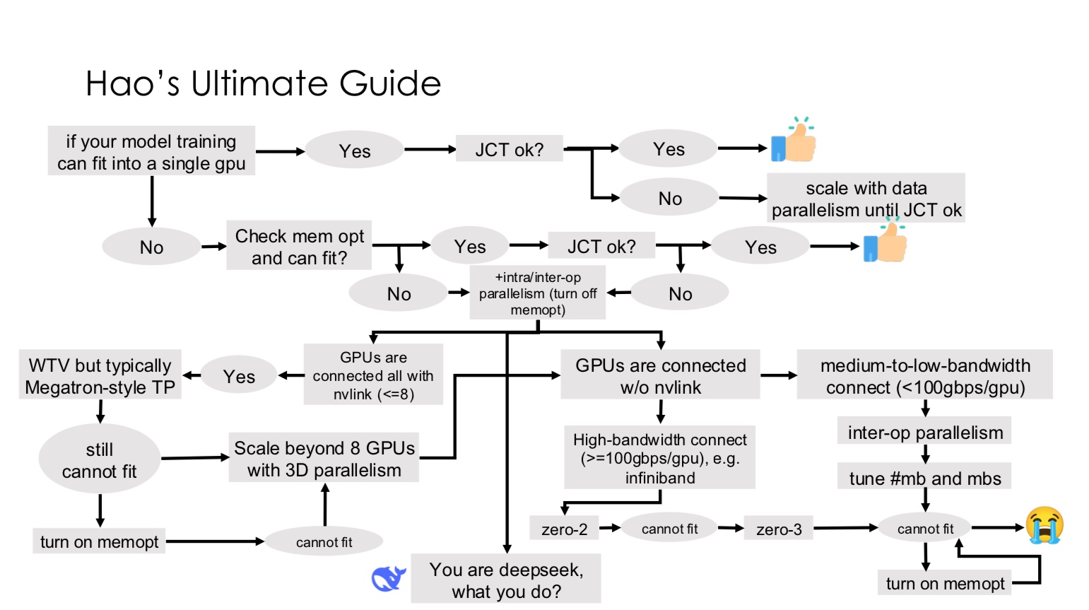
What is 3D parallelism?
Connecting dots…
We have studied all the concepts. Let us know see how they are used in practice.
A bit of refresher
We’ll list out all aspects of an LLM that are relevant for implementation -
LLMs do next-token prediction. They basically do Maximum Likelihood Estimation based on the tokens given so far (with the prompt or generated). Transformers at their core are seq2seq NNs built on top of attention mechanism.
The attention score computes how relevant the position i’s token is to a given output token. With language, we choose the same tokens for input and output (hence, self-attention).
\[SelfAttention(Q, K, V) = \text{softmax} \left(\frac{QK^T}{d^{1/2}\right) V\]Conceptually, we perform this calculation in two steps -
- Pre-softmax attention score $$s_{ti} = \frac{1}{\sqrt{d}} q_tk_i^T
- Weighted average via softmax - $$h = \sum_i \text{softmax}(s)_i v_i
We also have multiple attention heads in models to calculate different features. We get \(Q, K, V\) using embedding layers \(W_Q, W_K, W_V\).
During training, we also mask the attention so that a causal relation is maintained. Only attend to previous tokens. In naïve implementation, we make the entries of the attention matrix corresponding to the mask negative infinity. Can we be more smart about them and skip these calculations? Turns out masking later is more efficient due to GPUs behavior we’ve seen before - oversubscribe and don’t disturb the layout!
Given all this, we summarize the following
- Self-attention is slow
- Layer-norm, residual - fast
- MLPs - slow
- Non-linear activations - fast
- Word and position embeddings - fast
- Loss function - fast
So from a computing perspective, how do we make self-attention fast?
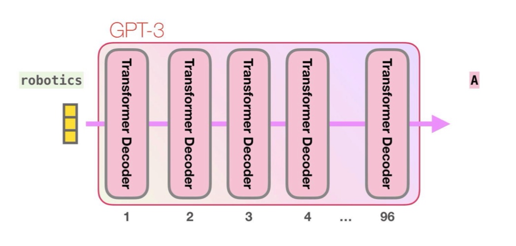
GPT-3 has 96 of these! So we definitely need to make it fast.
These were the core parts of an LLM. Notably, only the fast operations have been changing a lot, and the core attention and MLP mechanisms have remained.
| Feature | Vaswani et al. | LLaMA |
|---|---|---|
| Norm Position | Post | Pre |
| Norm Type | LayerNorm | RMSNorm |
| Non-linearity | ReLU | SiLU |
| Positional Encoding | Sinusoidal | RoPE |
Training LLMs
As we have noted, the three main components of implementation are compute, memory and communication. We must know
- The number of parameters of an LLM - it tells us how much memory and communication bandwidth is needed
- The FLOPs needed to train the LLM - it tells us how much compute is needed
- The memory needed to train an LLM - again, tells us about memory and communication considering activations and gradients
Let us delve into each of these questions
Calculating number of parameters
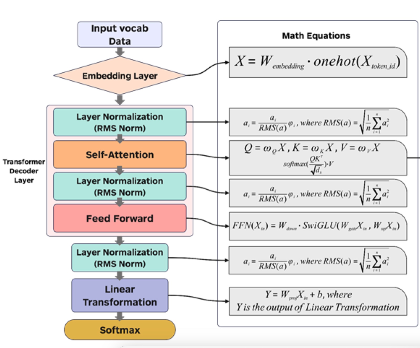
- The embedding layer has weight matrices of size $$
-
The SwiGLU layer has the following equation
\[\text{SwiGLU}(x) = \text{Swish{(xW_1 + b_1) \cdot (xW_2 + b_1)\]So in comparison with vanilla feedforward, we have one extra set of parameters.
- The linear transformation in the end essentially converts embeddings to token space and shares the weights with the embedding layer (
tie_embdin HuggingFace)
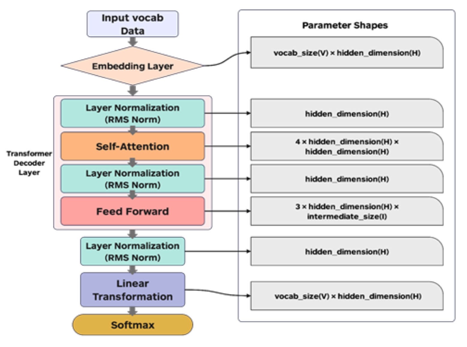
Notice that the major bottleneck comes from the feedforward layers. It has \(12h^2\) parameters in LLaMa! The second bottleneck is from self-attention which has \(4h^2\) parameters.
Calculating FLOPs
As we’ve noted multiple times, matmul is the most expensive operation in terms of FLOPs. We’ve seen that the total number of FLOPs is approximately \(2mnh\) for multiplying matrices of sizes \((m \times n)\) and \((n \times h)\).
| Component | Output Shape | FLOPs |
|---|---|---|
| Input: | ||
| X | (b, s, h) | 0 |
| Self Attention: | ||
| XW_Q, XW_K, XW_V | (b, s, h) | 3 * 2bsh² |
| RoPE | (b, n, s, d) | 3bsnd |
| P = Softmax(QKᵀ/√d) | (b, n, s, s) | 2bs²nd + 3bs²n |
| PV | (b, n, s, d) | 2bs²nd |
| AW_O | (b, s, h) | 2bsh² |
| Residual Connection: | (b, s, h) | bsh |
| Output from Self Attn: | ||
| X | (b, s, h) | 0 |
| Feed-Forward SwiGLU: | ||
| XW_gate / XW_up | (b, s, i) | 2 * 2bshi |
| Swish Activation | (b, s, i) | 4bsi |
| Element-wise * | (b, s, i) | bsi |
| XW_down | (b, s, h) | 2bshi |
| RMS Norm: | (b, s, h) | 4bsh + 2bs |
where
- b: Batch size
- s: Sequence length
- n: Number of attention heads
- d: Hidden state dimension of one head
- h: Hidden state dimension
- i: SwiGLU projection dimension
Note that attention is a very expensive operation because we have \(s^2\) - it does not allow us to scale to large number of tokens!
The final equation we get is
\[\text{Total FLOPs} = \#\text{num layers} *(6bsh^2 + 4bs^2h + 3bs^2 n + 2bsh^2 + \#\text{num layers} (6 bshi) + 2bshv\]For Llama 7B, this comes out to be 63 TFLOPs! The MLP is \(\approx 55\%\) of the total FLOPs and attention is \(\approx 41 \%\)!
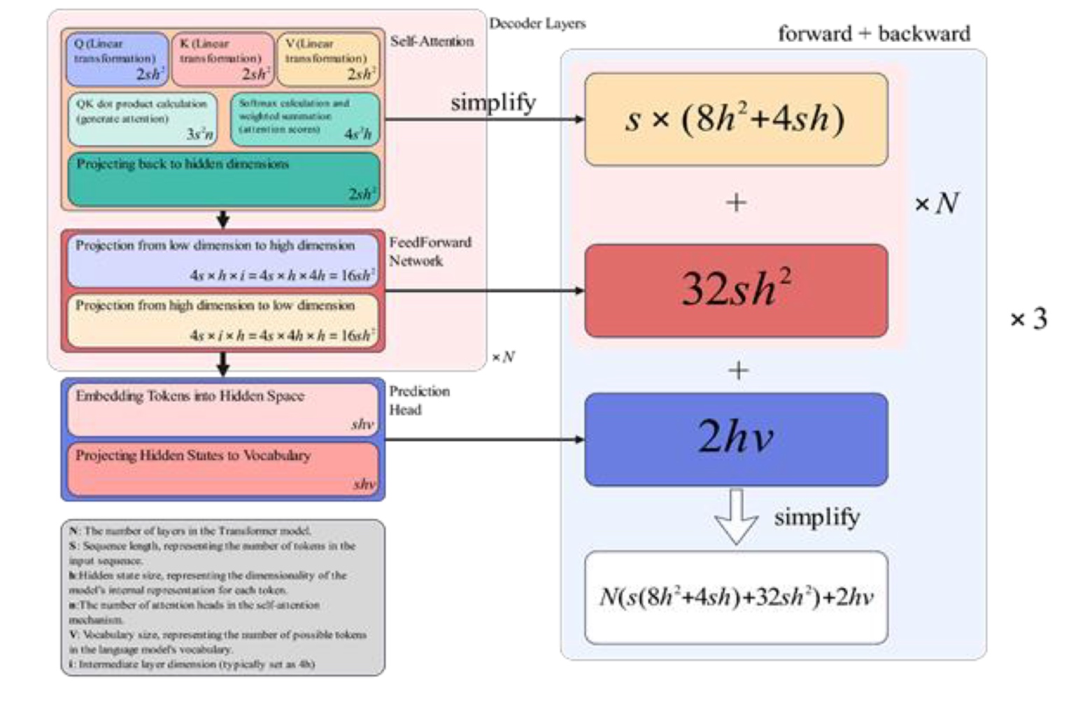
To reduce the bottleneck, one might try to decrease \(h\) (the hidden dimension) to scale up the model. The other way is to reduce the sequence length.
Note the factor of 3 above that is because of training (the model parameters and optimizer parameters). Let us recall the memory usage in models
- Model Weights - \(2 \times M\) for FP16
- Intermediate activation values
- If we checkpoint at transformers boundary, the activation memory is \(b \times s \times h \times n\_layers\). It is same as what we need to communicate in inter-op parallelism.
- The activation inside a transformer has the size \((b, n, s, s)\). It is the bottleneck for memory! We’ll see Flash Attention on how to avoid saving the complete attention matrix
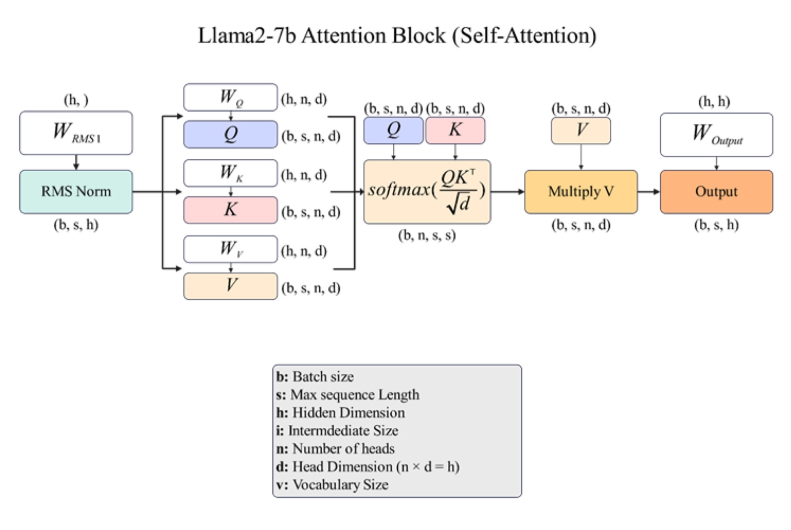
In summary, these are the activations inside the transformer block.
- Optimizer State - \(12 \times M\) for FP16-32 mixed-precision
- Weight Gradients + Activation Gradients - \(2 \times M\).
Based on this analysis, we have the following observations
- All terms are at least linear with \(h\) - Useful observation for scaling up
- Dimensions of partitioning
- \(b\) would be data parallelism
- \(d\) - Megatron based architecture
- \(s\) - Part of 4D parallelism
Advanced Topics (Recently published research) Megatron-style parallelism has been well adapted. How do we partition along \(s\)? We can partition \(n\) is attention (assign different heads to different GPUs) and \(s\) in MLP. Deepspeed Ulysses sequence parallelism is a recently proposed technique that partitions on \(n\) first and then partitions on \(s\). Moreover, it often happens that \(n \ll \#GPUs\) or is not a multiple of 8, then it is prudent to partition \(s\) in both attention and MLP. This is implemented in the form of ring attention.
Rule of thumb: In many computer systems and algorithms, anything more complex than quadratic is less likely to be adapted at large scale.
Scaling Laws
Continuing on our observations
- Computer is a function of \(h, i, b\)
- \(\#\)parameters is a function of \(h, i\)
- So the computer is a function \(\#\) parameters.
But as we know, the compute budget is limited. Then we have to decide between
- Training models longer (on more data) vs training bigger models
- Collect more data vs get more GPUs
- How to choose exact \(h, i\), etc.
Our motivation for scaling laws is to understand how large a model should we train and how much data should we use to achieve a given performance subject to a compute budget.
For applications like statistical estimators, we can easily derive theoretical scaling laws based on mathematical axioms. However, that seems to be much difficult for language models.
Then, how do we analyze these models? We perform empirical observations. Our analysis on machine learning has moved from mathematics based proofs to physics like experiments. Relying on observations. It became a strong trademark after the GPT-3 paper.
Here is what we have got so far, observing based on empirical scaling laws:
- To conclude transformers are better than LSTMs, instead of spending tens of millions to train LSTM GPT-3, we extrapolated results and noticed that transformers outperform these models.
- Similarly for depth vs width of networks - 1 vs 2 layers make s a huge difference but more layers have diminishing returns after a certain number of parameters.
Essentially, the scaling law way trains smaller models to establish a scaling law and select the optimal hyper-parameters based on the scaling law prediction. This allows us to get a heuristic on the effects of hyper-parameters in big LMs before training.
Consider the question data vs compute trade-off - for a given compute is it better to train undertrained big models or well-trained small models?
\[N_{opt} (C), D_{opt}(C) = \arg_{N, D}\min_{FLOPs(N, D) = C} L(N, D)\]where \(N\) is the number of parameters, \(D\) is the data and \(C\) is the compute. We obtained the following after spending billions of dollars for next-prediction loss
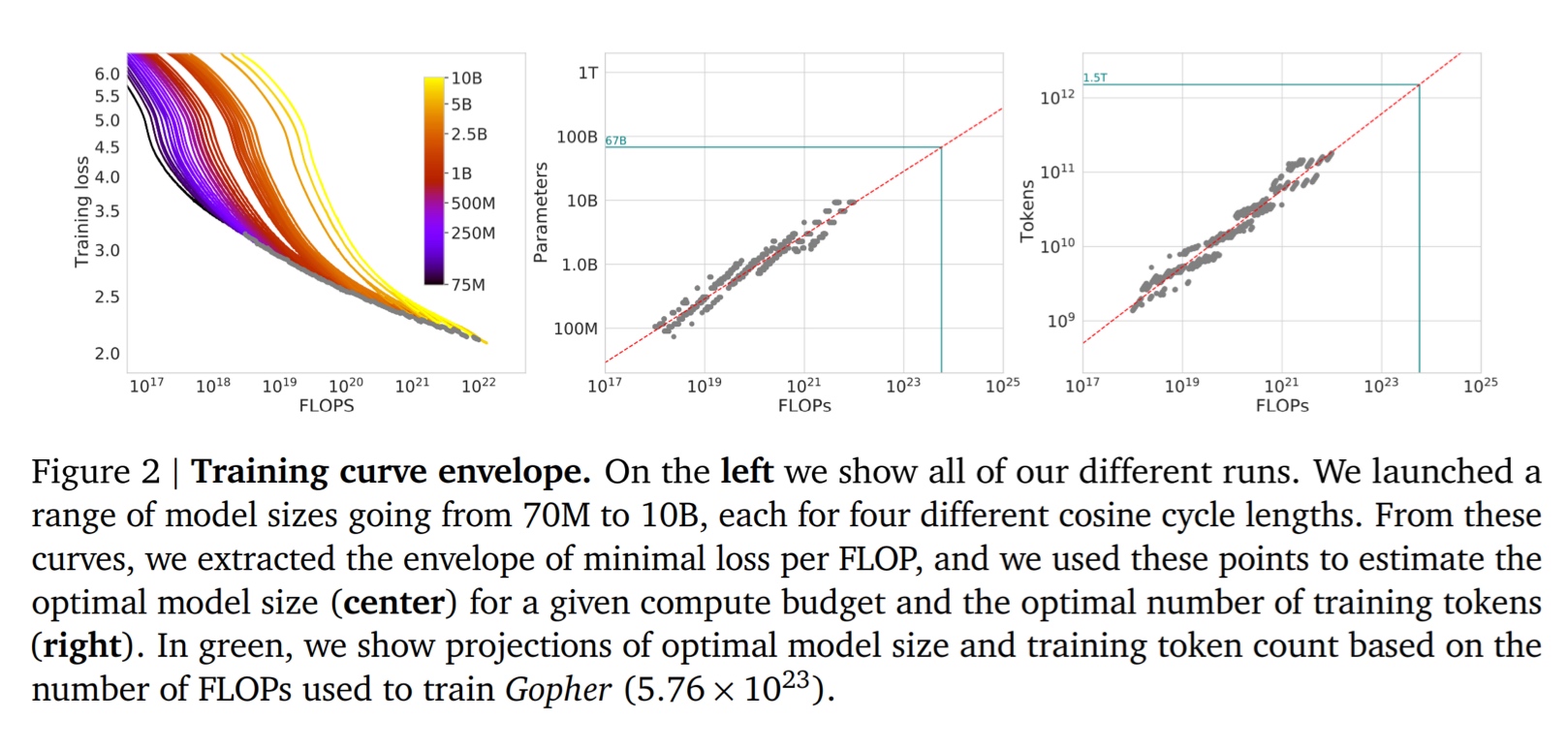
and every LLM seems to follow this…
MoE LLMs
The key idea like we discussed before is to make each expert focus on predicting the right answer for a subset of cases.
Instead of choosing one expert each time, it is also possible to choose multiple experts for a token, and that becomes another hyper parameter. That is, we can choose to activate two experts each time and add the output of both of them.
Let us consider the number of parameters and analyze MoE with scaling laws.
- The number of parameters increase drastically - MLP params \(\times N/2\) (if we choose to activate 2 experts each time) where \(N\) is the number of experts. For example, Deepseek V3 has 256 experts!
- Memory for parameters increases by the same factor. However, activations don’t consume too much additional memory. Even though the parameters increase drastically, the compute only increases mildly. This is why Deepseek blew up. For much higher number of experts, the attention parameters decrease largely (sparse activations in experts), and they were able to train dense model equivalent model with much lower compute.
People also tried to get scaling laws for MoEs and noticed that MoE is a much more compute-efficient model (it has a better scaling law).
Let us analyze the architecture again. We stuck to a Megatron like architecture for transformers. However, it would not work with MoE since all the weights are replicated number of expert times. So we perform parallelism in the dimension of experts. 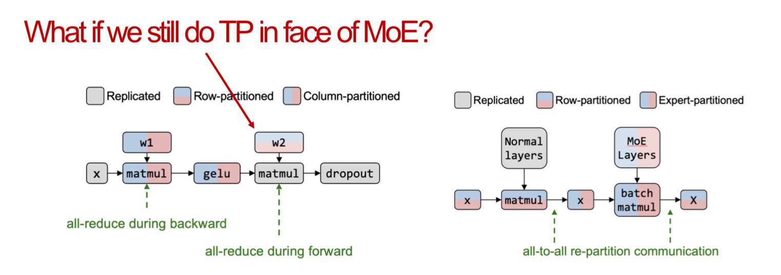
This way, each GPU would have different workloads (bubbles!) - A hot expert problem. Deepseek implemented many mechanisms to reduce this as much as possible.
Inference
So far we’ve studied that LLMs are slow and expensive to serve. At least 10 A100-40GB GPUs are required to serve 175B GPT-3 in half precision and generating 256 tokens takes approximately 20 seconds.
The key factor is that we perform autoregressive decoding - we require the current token to predict the next token. Note that we predict until the pre-defined maximum length or we reach the end of sequence.
The inference stage can be divided into two stages
- Prefilling - Process all input tokens at once (prompt)
- Decoding phase - Process a single token generated from previous iteration (generating)
The decoding phase is optimized with Key-value cache by saving attention keys and values during the decoding phase to avoid recomputations.
In a broader sense, serving an LLM has more considerations during inference. For a larger group, it would be prudent to emphasize on throughput and if it is an individual then latency is a concern. How do we optimize for these scenarios?
Different techniques have been proposed. For the single user case, a popular technique has been speculative decoding.
The latency is essentially \(\text{latency} = \text{ step latency} \times \#\text{steps}\)
With speculative decoding, we try and reduce the number of steps!
[Guest Lecture: Hongyang Zhang] Speculative Decoding
The vanilla autoregressive inference involves sampling tokens from a probability distribution that is obtained by the tokens generated so far.
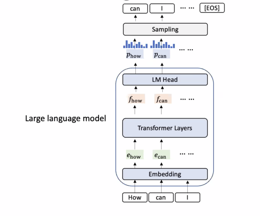
How do we move from this sequential sampling framework to a parallel one?
Speculative sampling framework (introduced in Leviathan et al) uses a much smaller model that is a good approximation of the original large model. This tiny draft model is used to create a draft of the response in the same sequential autoregressive manner. Since the model is tiny, the inference is faster.
The tokens generated by the draft model are fed into the LLM to generate the distributions from these tokens in parallel. The draft model can be verified by comparing the distributions of both the models for a given token.
-
We generate a number \(r\) between 0 and 1 uniformly, and check if \(r < \min(1, p(t)/q(t))\) where \(p\) is the LLM distribution and \(q\) is the draft model distribution.
-
If the condition holds, we accept the token. Otherwise we correct the token by sampling \(t' \sim \norm(\max(0, p - q))\). All the tokens following this corrected token are discarded, and the process is repeated again.
There is theoretical work that shows that the above procedure is equivalent to sampling from \(p\).
Given this, how do we build the tiny model \(q\)? That is the crux of the methods in this domain.
Does this framework only work for greedy sampling? No, it can be extended to non-greedy sampling techniques with some modifications.
The tiny model used can have low rejection rates for tasks like summarization but may have high rejection rates for tasks involving reasoning. So, there’s a trade-off with the draft model overhead and the rejection rate.
Building \(q\) with EAGLE-v1
As mentioned before, building \(q\) is a trade-off between accuracy and efficiency. They have proposed EAGLE.
The authors of this paper observed that the initial distribution of the embeddings in the initial layers is very complicated and dynamic. However, for the top layers, the distribution becomes much simpler - that is, the distribution to predict next tokens from previous tokens.
So, they tried to estimate the features rather than the tokens directly. In their first attempt, they trained a single transformer layer to learn the embeddings (features) in the last layer of LLMs. Essentially, instead of using the first layer tokens, they used the last layer features for the speculative decoding framework. With this, they obtained a much higher speed-up and accuracy!
However, they noted that this model does not use feature uncertainty correctly. In the speculative decoding framework, the parallel decoding in the large LLM does not consider the previously generated
To solve this, they tried another method by predicting the distribution by concatenating the initial token embedding with the feature from the last layer. They attribute this as adding a shifted token embedding.
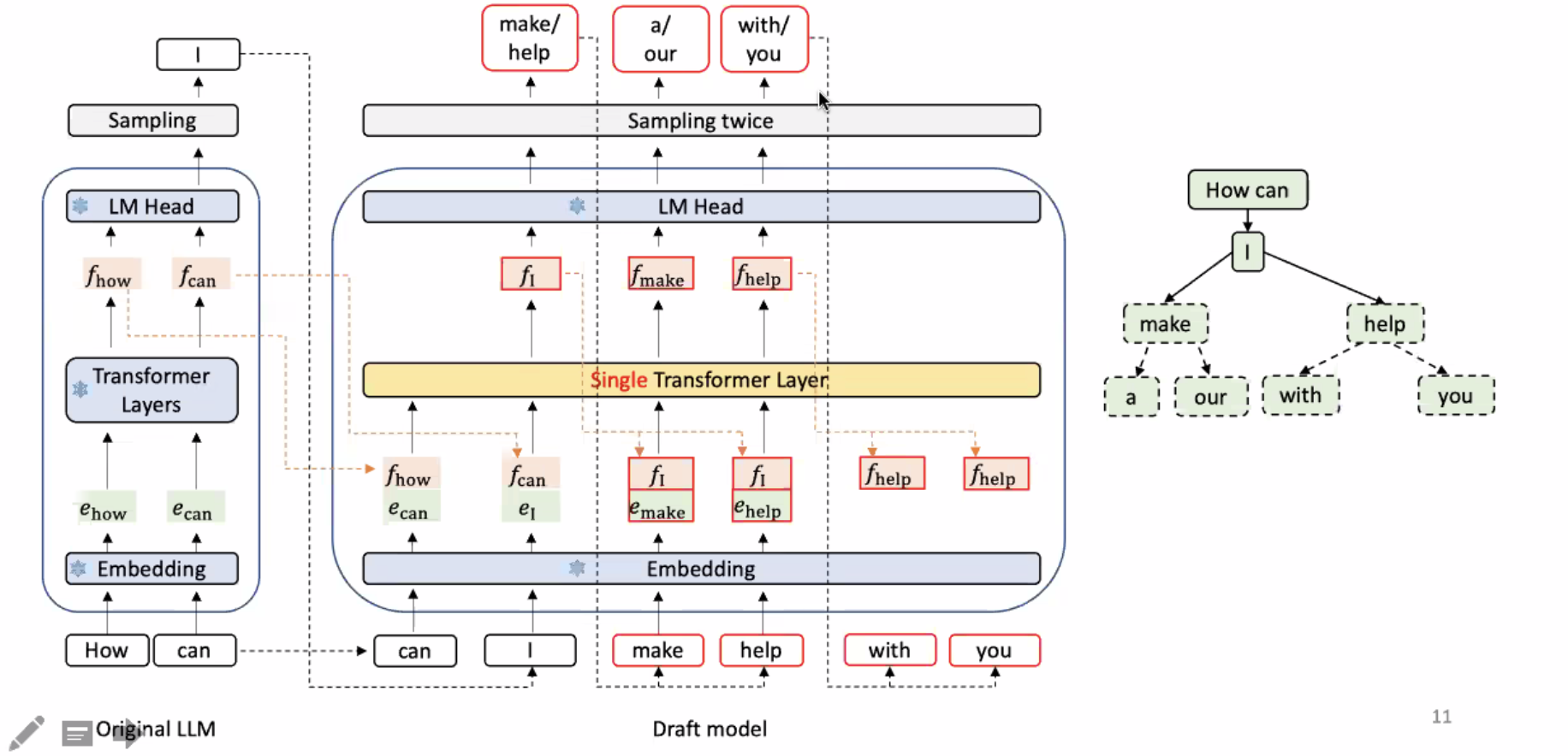
Essentially, we generate choices through the draft model rather than a single prediction. With this, we obtain a much higher speed-up and accuracy -
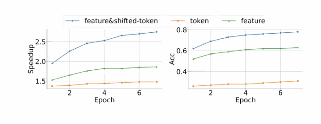
Note that the attention mask for thi has to be carefully design as follows -
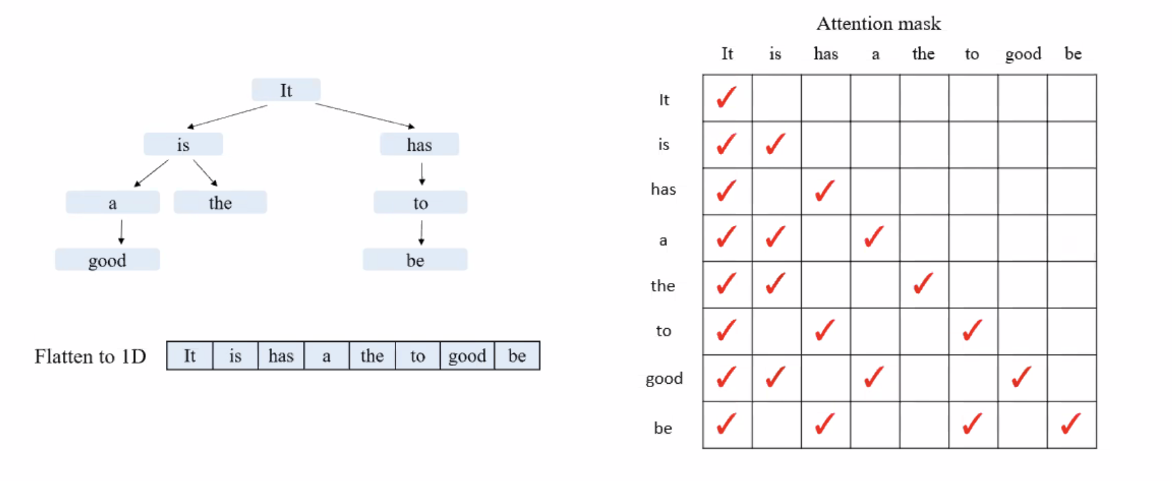
Because of this, the model cannot handle long-context settings.
The draft model can be around 1-3% (higher percentage for smaller models to account for the dimensionality of the latent space) of the larger model leading to a very high speed-up!
EAGLE-v2
The authors noted that the method can be improved even further. They noted that the accuracy of the speculative decoding tree if higher to the top-left and lowest to bottom-right. So, they associated a confidence score to each node in the tree. Ideally, that would be \(\min(1, p(t)/q(t))\), but they found that \(q(t)\) is a good approximation and has a strong linear correlation with the actual quantity.
With this, they build a context-aware dynamic draft tree.
Essentially, instead of generating a tree, they do beam-search with the small model.
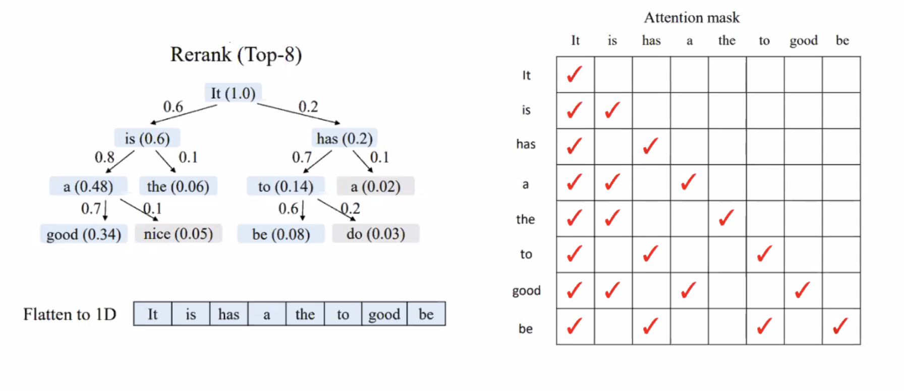
As expected, this method obtained even higher speedup and accuracy!
They didn’t stop there.
EAGLE-v3
They published yesterday lol! With the new method that has a modified training routine and a loss function, they noticed a new scaling law that seems to perform better as the model grows. Essentially, they introduced draft model inference in the training routine to better simulate the inference routine.
They also observed that the performance is the best when the draft model architecture is the same as the large model.
The draft model just generates a draft and not the complete response. For example, it will generate 6 words, and these are used by the larger LLM. So it’s different from knowledge distillation.
Getting back to our context, let us talk about LLM inference.
We mentioned KV-cache before - It stores the previously calculated attention values during the next-token generation to reuse the values -

There are issues with this approach is
- Compute: The arithmetic intensity in the GPU is decreased, and GPU may be under-utilized. When \(n = 1, s = 1\), the GPU is underutilized.
- Memory: Need to store KV cache until the request is completed
- Communication: Mostly same
Note that the batch size during inference is dependent on the application request load - It is a tradeoff between efficiency and latency reduction as we have mentioned before. We have also seen how speculative decoding is used to decrease the latency in case of single requests. Now, we will consider the other side - how do we handle a large number of requests while keeping the cost-per-query less. Let us again consider the three elements to find the potential bottleneck during inference
- Compute:
- Pre-fill - Requests have different lengths. How do we batch?
- Decode - We do not know the number of tokens that need to be generated ahead of time.
- Memory: KV-Cache is an issue for these large batch sizes.
- Communication: Remains the same.
Recent works have addressed these issues, and the requirements for LLMs have almost decreased \(60 \times\). Speculative decoding does not work for large batch sizes - it is being explored in research currently.
Continuous Batching
Suppose we have two prompts that are passed to the server.
- We cannot batch the sequences for attention if they have different number of tokens. So, here arises a crucial loss in performance - whether to pad all the short requests to make everything equal.
- However, since MLPs are token independent, the requests can be batched! No loss in performance here.
Due to this difference, the current implementations perform cyclic batching and de-batching to execute attention of different requests on different ranks, and then merge all requests to get the MLP output.
Suppose a new request enters while the earlier requests are being processed - the new request can be easily be batched for the MLP phases after the attention has been calculated separately. In standard pipelines without continuous batching, such behavior is not allowed - a batch is issued and run until completion. A new request in the queue cannot enter and a request that finished early cannot exit.
Recall that when we calculated the FLOPs for a transformer, the MLP requires the maximum number of FLOPs. So, batching these stages results in huge gains in performance.
Note. The pre-fill and decoding phases for attention are superficially the same for this setup - they are separately calculated on each kernel before being batched for MLP passes.
So essentially, we have introduced a lot of flexibility into transformer forward passes which were previously treated as atomic. We have improved GPU utilization with two key insights
- Attention consumes small percentage of FLOPs for medium context
- MLP kernels are agnostic to sequence dimension
KV-Cache Key Insight
KV Cache needs to be efficiently managed for high-throughput LLM serving. The KV Cache can become super large for long sequences.
 The throughput of the GPU is proportional to the batch size. That is, the execution time for 40 batches would be same as that of 8 batches because of how a GPU functions!
Note. Why is the throughput higher for higher batch sizes?
So, if we can reduce the memory usage of KV-Cache, we can process more batches in the same time! How do we do this?
- Internal Fragmentation - Memory for KV Cache is over-allocated because we do not know the output length.
- Reservation - Memory that is not used at the current step (but will be needed in the future) is wasted

There is also external fragmentation that demarcates areas of different requests. Due to all these different things - only 20-40% of KV cache is used to store the tokens!!
vLLM - Paged Attention
Drawing inspiration from virtual memory and paging in the OS, we improve how we store the values in KV cache.

Deep-learning workflows typically consider contiguous blocks of memories. Breaking that standard, we store KV cache using continuous keys and values in non-contiguous memory space. Similar to OS mechanisms, we use logical and physical token blocks connected through a page table. Refer to my notes on OS to understand these better.

Through this, we allocated memory on demand and minimize the internal fragmentation! We use CPU to orchestrate all this. There is no external fragmentation at all! With this, we have the following results -

Prefill-decode disaggregation
To better benchmark LLM-based services, we consider new service based metrics
- TTFT - Time to first token For a chatbot, we need to have fast initial response. For tasks like summarization, it can be slower.
- TPOT - Time per output token Generate as fast as human reading speed for chatbots. For summarization, needs to be super fast.
Any requests completed within Service Latency Output (SLO) are factored into goodput. High throughput can still have low goodput. We discussed continuous batching, but it has the following limitations
- Prefill - Compute bound, one prefill saturates compute.
- Decode - Memory bound, need to batch many requests together to saturate compute.

To prevent these limitations, the idea of disaggregating prefill and decode phases has been proposed - Essentially, the prefill and decode steps are performed on different GPUs. There is an overhead of communication to transfer the KV cache from prefill phase to the decode phase, but the requests can be processed in parallel increasing the throughput. The result of this can be seen below -
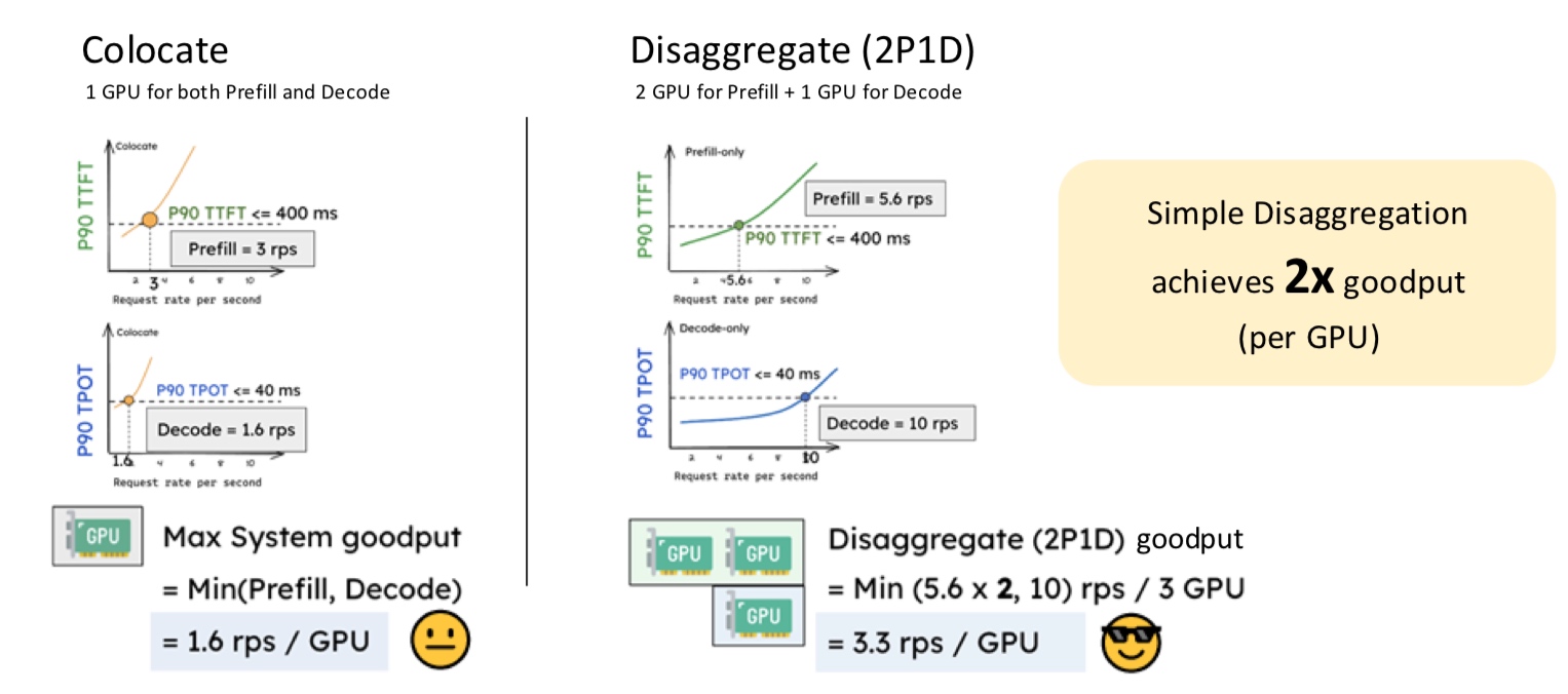
The curve for decoding in the disaggregate system is flatter since there is no prefill phase competing for resources.
This system became a norm in the past few months. Deepseek-v2 uses prefill-decode disaggregation combined with different parallelisms for prefill and decoding instances.
Furthermore, continuous batches and disaggregation are actually orthogonal to each other (doesn’t seem so at the first glance)
- Continuous batching improves GPU utilization and hence the throughput
- Disaggregation addresses goodput such that SLOs are satisfied
The key insights from CB still carry to disaggregation.
LLM Inference is a very hot research topic right now. We have seen many techniques from this field
- Scheduling - continuous batching, chunked prefill, disaggregated prefill and decoding
- Speculative Decoding
- Memory bottleneck of KV Cache - new attention mechanisms - paged, sparse, etc and sparse KV cache
- Kernel optimizations
With that, we move to the final topic of this article.
FlashAttention
Coming back to the computations in the transformer, we saw that the attention operation is limited by the sequence size (proportional to \(\mathcal O(n^2)\)).
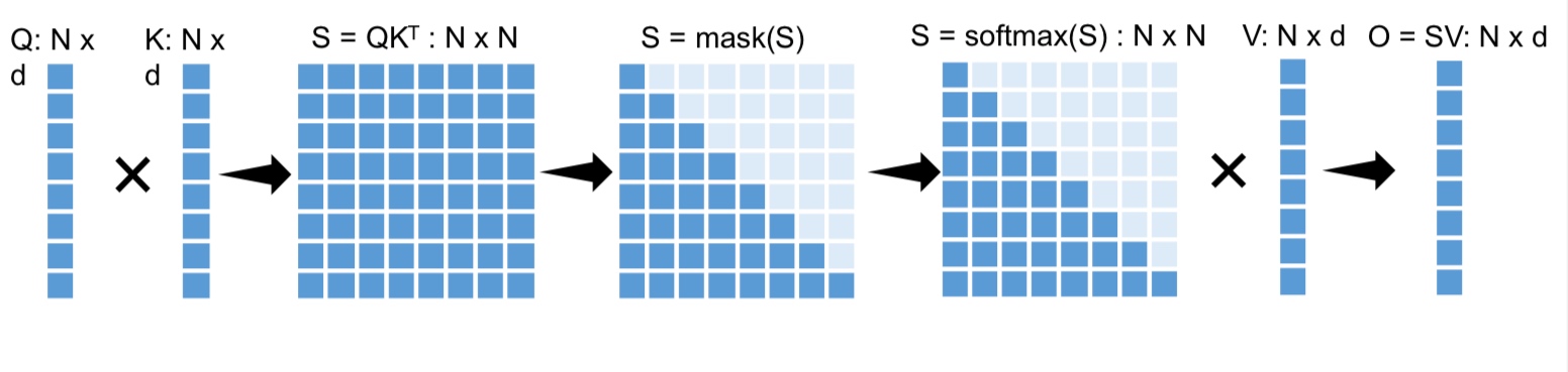
The internal matrices have sizes proportional to square of the sequence length and we have to materialize these matrices. That is, we explicitly compute and store these matrices. Putting this into perspective with numbers we have
For \(b = 1k, n = 32, h = 4k, s= 4k\),
- Memory = \(bs^2n = 512Gb\)
- Compute = \(4bs^2h = 256 TFLOPs\)
The GPU memory is much more scarce than compute with our current hardware. Is there a way we can reduce the memory usage to improve the attention block?
The implementations before FlashAttention explicitly calculated the internal matrices and moved them between HBM and kernel SRAM. These repeated reads/write add a lot of latency.
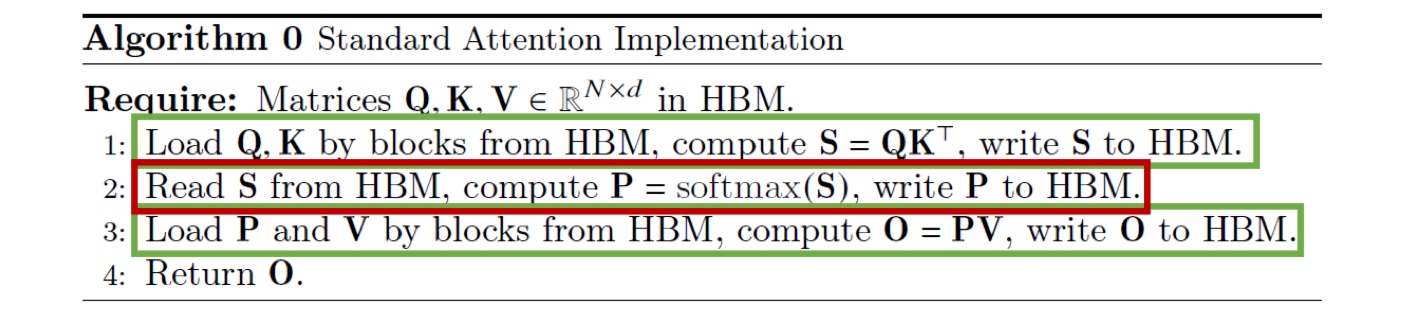
The issue arises due to the softmax operation. It is not trivial to calculate the final softmax output without the intermediate matrices. Furthermore, the backward pass also needs to be done without the intermediate activations.
We were able to calculate matrix multiplication results without materializing the complete input and output. Can we do the same here?
Let us understand softmax first. Softmax is usually implemented in a numerically stable manner.
\[y_i = \frac{e^{x_i - \max_{k = 1}^V x_k}}{\sum_{j = 1}^V e^{x_j - \max_{k = 1}^V x_k}}\]This introduces another level of complexity for calculating the attention output. We observe the following relation while iterating through the array elements to find the softmax
\[\begin{align*} d_i &= \sum_{j = 1}^i e^{x_j - m_i} \\ d_i = d_{i - 1} e^{m_{i - 1} - m_i} + e^{x_i - m_i} \end{align*}\]Now, we observe that the final output can be represented as a recurrence depending on some precomputed values. We move from two loops (one for maximum and one for exponentiation) to one single loop for softmax based on the recurrence relation. It is known as online softmax calculation.
How do we use this to optimize attention?
If we can find some recursion structure in \(o\), we can use it to optimize attention by preventing explicit calculation of \(a\), and fuse the two loops together.
\[\begin{align*} o’_i &= \sum_{j = 1}^i \frac{e^{x_j- m_i}}{d_i’} V[j, :] \\ &= \cdots \\ &= o’_{i - 1} \frac{d’_{i - 1} e^{m_{i - 1} - m_i}}{d’_i} + \frac{e^{x_i - m_i}{d_i’} V[i, :] \end{align*}\]Voila! That gives us FlashAttention
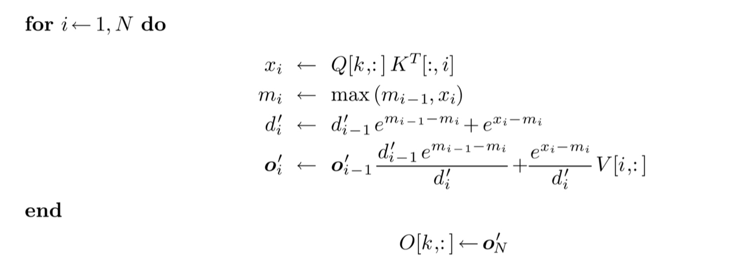
We never materialize the intermediate results, and transfer the matrices only once. That gives a huge speed up! FlashAttention also has tiling to utilize the GPUs to their fullest.
What about the backward pass? FlashAttention resorts to recomputation of required results instead of storing the activations, and this still gives a speed up! That is how memory-bottlenecked we are.
Overall, the method offers 104x speed up and 10-20x memory reduction!
FlashAttention got very successful because it has a cascading effect. Due to this method, we were able to train with larger batch sizes leading to much higher throughput (better AI). Also, the cost of training decreased significantly because we can now turn off gradient check pointing (no need to save memory anymore).
The method was further developed to FlashAttention2 and FlashAttention3 with more kernel-level optimizations with more aggressive fusion and memory access patterns. The success of FlashAttention is because of its unique insight into an opportunity that was created due to hardware limitations and rise of popularity of self-attention.
Connecting everything!
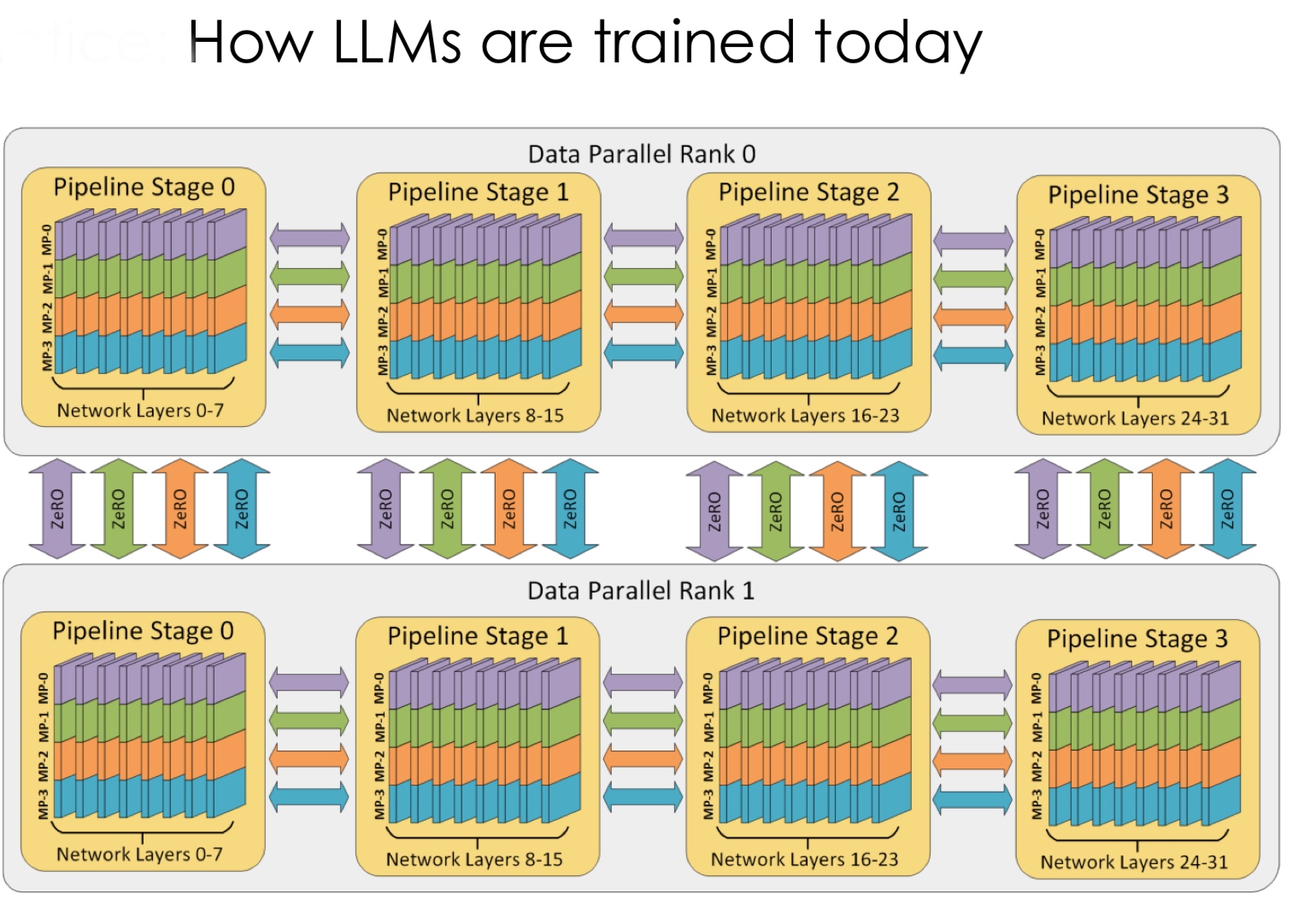
- Outer Loop 1: There is inter-op parallelism with pipelining such as 1F1B
- Outer Loop 2: There is intra-op parallelism based on model architecture (Zero-2/3 and data parallelism or Megatron-LM tensor parallelism)
- Outer Loop 3: Gradient check pointing and recomputation at backward pass
- Inner Loop 4: Graph Fusion
- Inner Loop 5: Operator-level optimization: tiling, flash attention, etc
Deepseek-v3!
Deepseek-v3 was the first open-source model that reached the performance of GPT-4o! This was a big feat.
Furthermore, they also made a bold claim of training the model with 100x lower cost! Many people argued that this is not a responsible claim since most of the budget is usually spent on the planning phase and not on the actual training phase. Previously it was all experimenting, and by the time Deepseek-v3 came into picture, many of these practices were set into stone. Either way, it was a big feat.
Model Architecture
People were familiar with Llama before this, but Deepseek had fundamentally changed things from minute-details to large architectural decisions. Firstly, they went big on Mixture-of-Experts (MoE). Companies usually chose 8-10 MoEs in models, and Deepseek went ahead with 256 experts! This decision while introducing new challenges, significantly made model training and inference much more scalable.
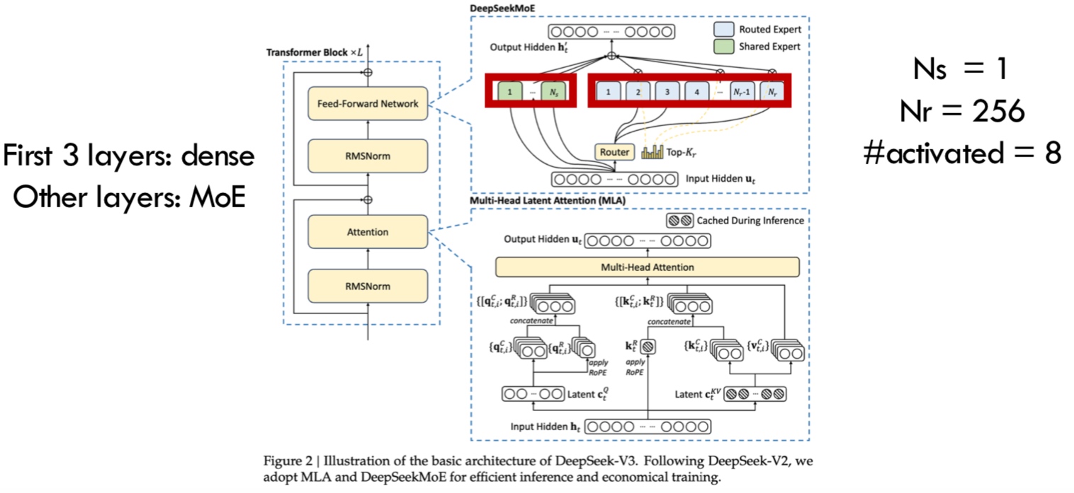
MoEs typically have much larger number of parameters requiring more communication between GPUs - we need expert parallelism with expert balancing.
They introduced a new kind of attention known as Multi-head Latent Attention (MLA) that reduced the inference cost by a huge amount.
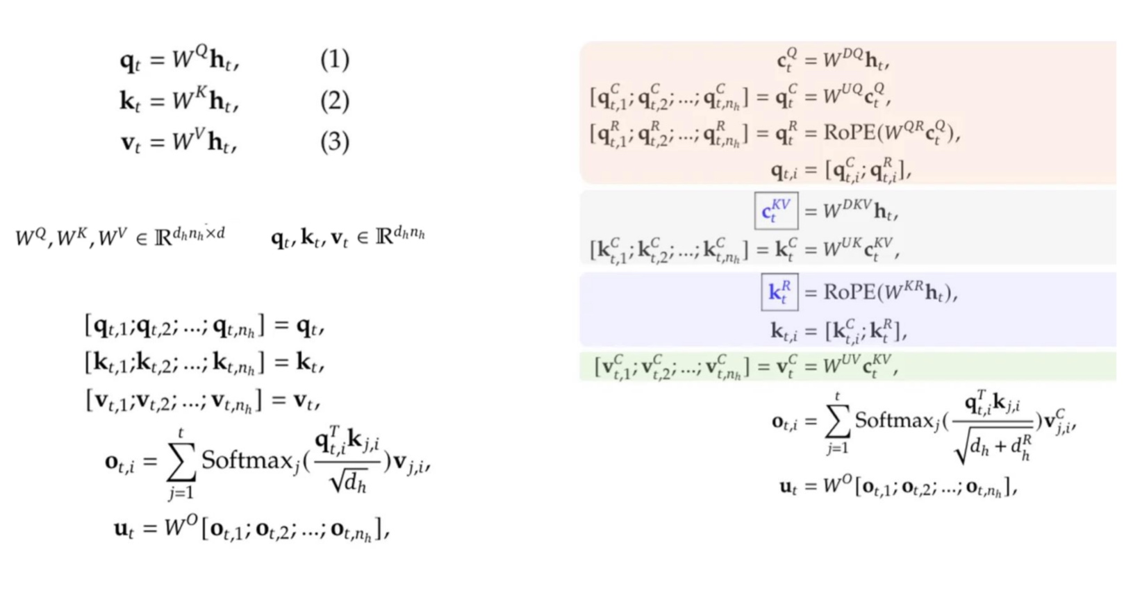
They introduced a new vector \(c\) that essentially stores the KV values in a low-dimensional latent space. This trades memory for FLOPs and significantly reduces the KV Cache per token.
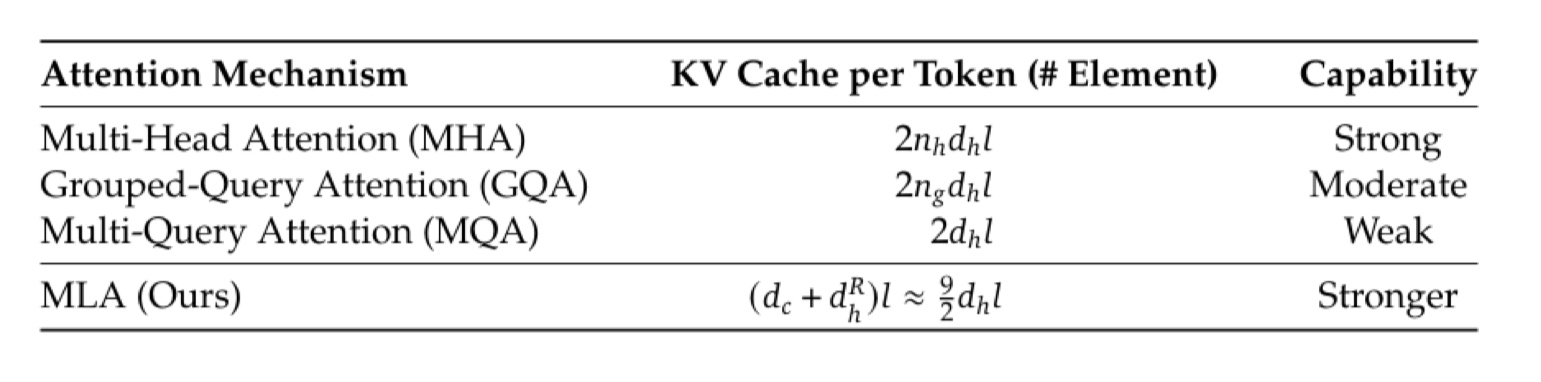
They claim that MLA has much stronger ML capabilities.
Another optimization in the model architecture is multi-token prediction. Inspired from the EAGLE series, they introduced speculative decoding in the pre-training phase. EAGLE claims 50% acceptance rate and the introduction of the speculative decoding into pre-training increases it to 80-85% acceptance! We essentially are getting a free speculation head.
System optimization
US infamously restricted the imports of the top NVIDIA GPUs (H100) to China, and Deepseek had to rely on a less powerful variant (H800) that does not have NVLink. Without NVLink, the communication overhead increases significantly. As a result, Deepseek cannot use tensor parallelism (all-reduce is \(N\times\) more complex than all-to-all). So they relied on pipeline parallelism, data parallelism and expert parallelism.
We have also seen the issues with expert parallelism - need to have a good balancing. Typically, systems add an expert balancing loss. Instead, Deepseek argues that this loss hurts the pre-training and they use an alternative auxiliary-loss-free bias term.
They use a sequence level balancing loss that encourages the expert load on each sequence to be balanced. (They said no loss but use another loss).
So, overall, they have 16 way pipeline parallelism, 64 way expert parallelism, and ZERO-based data parallelism. Assuming they have 2048 GPUs (which they claimed), they have 16 PP, 64 EP and 2DP for a total of 2048 GPUs. Note that in each stage of inter-op parallelism, we need two all-to-all for EP and only one all reduce for 2DP.
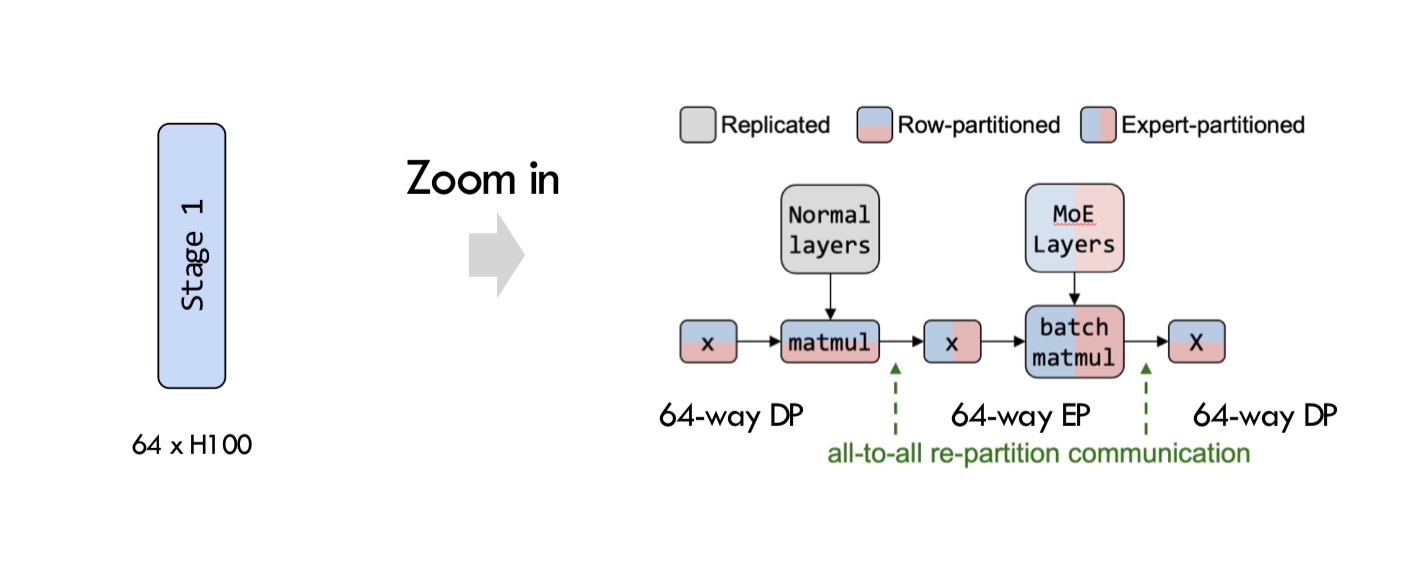 For pipeline parallelism, as we saw before, they introduced a new parallelism strategy on top of Chimera. Chimera required two copies of model weights in each rank. Chimera also has all-to-all communications that introduce some overhead. Let us look at the pipeline again -
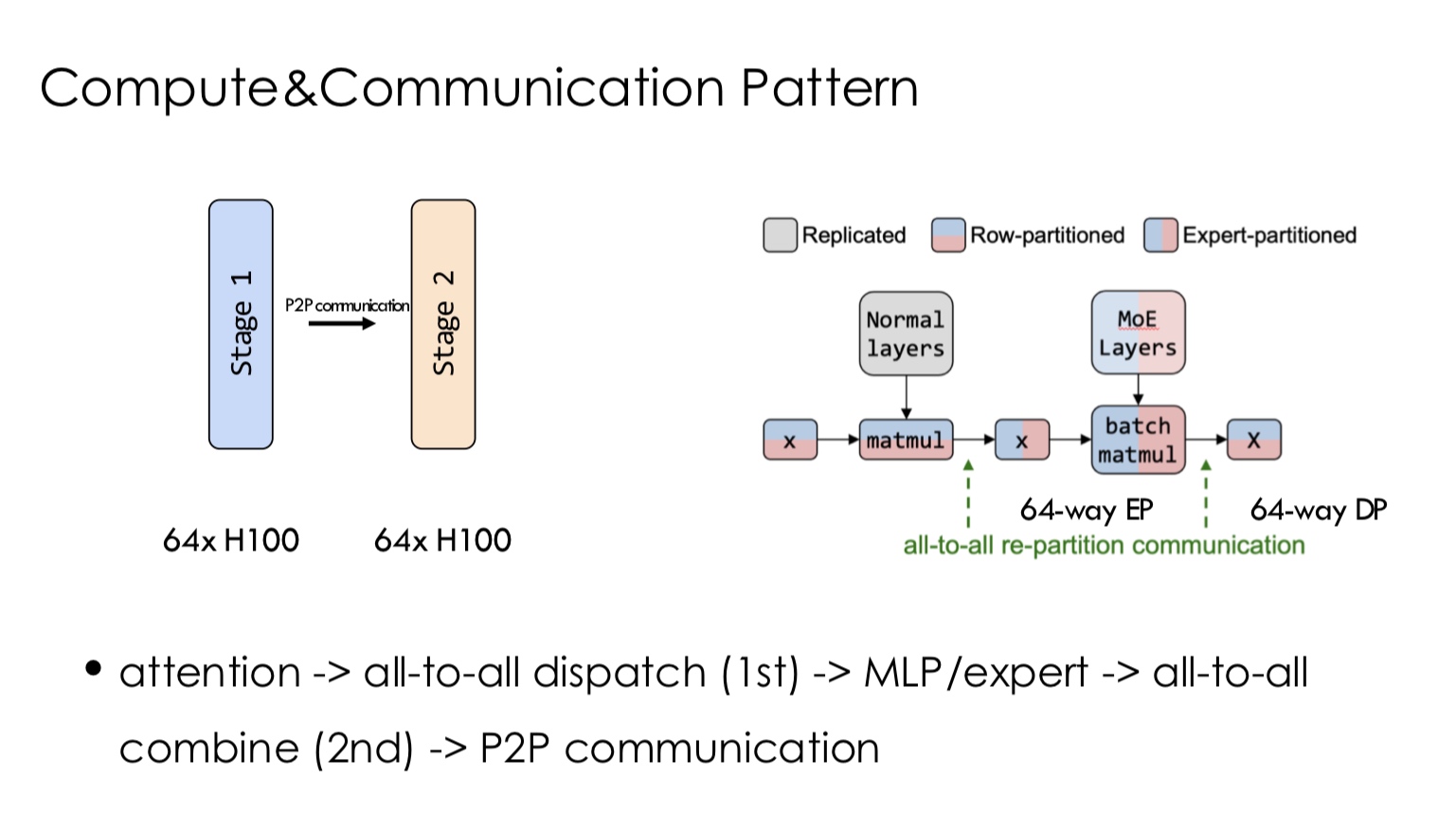
To top all this, they made their own All-to-all communication kernel that does some extreme optimizations.
Phew!
Final set of innovations
- They made their own mixed-precision training standard different from the rest of the industry that reduced the usage from \(16N\) (we’ve seen this before) to \(13N\) using FP8 tensor core.
- Even more fine-grained quantization for FP8 kernels
- Prefill-decode disaggregation based inference.
So, that is why Deepseek is big.
Conclusion
LLMs are big, we’ve said this too many times now. But LLM systems is getting even bigger, and there are innovations happening much much faster in all fields both because of new paradigms and AI helping humans becoming more productive. All this article content can be replaced in 1-2 years. So, us, as researchers or developers, need to be able to identify the right problems, the ability to understand trends and the ability to predict the future! Identify the right papers and invest in the right companies.
Enjoy Reading This Article?
Here are some more articles you might like to read next: