DiBS Notes
Lecture 1
03/01/2022
~Chapter 1: Introduction
- Embedded databases - Databases which don’t have high amount of concurrent access, but is mostly used by a single user. These databases are implemented by SQLite in general.
-
Motivation for Database systems -
- Atomicity
- Concurrency
- Security
- …
Data Models
A collection tools for describing the data, relationships in the data, semantics and other constraints.
We start using the relational models that are implemented using SQL. Then, we shall study Entity-Relationship data model. These are used for database design. We will briefly touch upon Object-based data models. Finally, we shall see Semi-structured data model as a part of XML.
There are also other models like Network model and Hierarchical model (old) etc.
Relational Model
All the data is stored in various tables. A relation is nothing but a table. Back in the 70’s, Ted Codd (Turing Award 1981) formalized the Relational Model. According to his terminology, a table is same as a relation, a column is also called an attribute, and the rows of the table are called as tuples. The second major contribution he made was introducing the notion of operations. Finally, he also established a low-level database engine that could execute these operations.
Some more terminology - Logical Schema is the overall logical structure of the database. It is analogous to the type information of a variable in a program. A physical schema is the overall physical structure of the database. An instance is the actual content of the database at a particular point in time. It is analogous to the value of a variable. The notion of physical data independence is the ability to modify the physical schema without changing the logical schema.
Data Definition Language (DDL)
It is the specification notation for defining the database schema. DDL compiler generates a set of table templates stored in a data dictionary. A data dictionary contains metadata (data about data) such as database schema, integrity constraints (primary key) and authorization.
Data Manipulation Language (DML)
It is the language for accessing and updating the data organized by the appropriate data model. It is also known as a query language. There are basically two types of data-manipulation languages - Procedural DML requires a user to specify what data is needed and how to get that data; Declarative DML requires a user to specify what data is need without specifying how to get those data. Declarative/non-procedural DMLs are usually easier to learn.
SQL Query Language
SQL query language is non-procedural! It is declarative. SQL is not a Turing machine equivalent language. There are extensions which make it so. SQL does not support actions such as input from the users, typesetting, communication over the network and output to the display. A query takes as input several tables and always returns a single table. SQL is often used embedded within a higher-level language.
Database Design involves coming up with a Logical design and Physical design.
A Database Engine accepts these queries and parses them. It is partitioned into modules that deal with each of the responsibilities of the overall system. The functional components of a database system can be divided into
-
Storage manager - Actually stores the data. It takes the logical view and maps it to the physical view. It is also responsible to interact with the OS file manager for efficient storing, retrieving and updating of data. It has various components such as authorization and integrity manager, transaction manager, file manager and buffer manager. It implements several data structures as a part of the physical system implementation - data files, data dictionary and indices.
-
Query processor - It includes DDL interpreter, DML compiler (query to low-level instructions along with query optimization) and the query evaluation engine.
Query processing involves parsing and translation, optimization, and evaluation. Statistics of the data are also used in optimization.
-
Transaction management - A transaction is a collection of operations that performs a single logical function in a database application. The transaction management component ensures that the database remains in a consistent state despite system failure. The concurrency control manager controls the interaction among the concurrent transactions to ensure the consistency of the data.
Lecture 2
04-01-22
Database Architecture
There are various architectures such as centralized databases, client-server, parallel databases and distributed databases.
~Chapter 2: Intro to Relational Model
Attributes
The set of allowed values for each attribute is called the domain of the attribute. Attribute values are required to be atomic - indivisible. Todd realized that having sets or divisible attributes complicates the algebra. The special value null is a member of every domain that indicates the value is unknown. The null values causes complications in the definition of many operations.
Relations are unordered. The order of tuples is irrelevant for the operations logically.
Database Schema - The logical structure of the database.
Keys
K is a superkey of the relation R if values for K are sufficient to identify a unique tuple of each possible relation \(r(R)\). Superkey \(K\) is a candidate key if \(K\) is minimal. One of the candidate keys is selected to be the primary key. A foreign key constraint ensures that the value in one relation must appear in another. There is a notion of referencing relation and a referenced relation.
Relational Query Languages
Pure languages include Relational algebra, Tuple relational calculus and Domain relational calculus. These three languages are equivalent in computing power.
Lecture 3
06/01/2022
Relational Algebra
An algebraic language consisting of a set of operations that take one or two relations as input and produces a new relation as their result. It consists of six basic operators -
- select \(\sigma\)
- project \(\Pi\)
- union \(\cup\)
- set difference \(-\)
- Cartesian product \(\times\)
- rename \(\rho\)
We shall discuss each of them in detail now.
Select Operation
The select operation selects tuples that satisfy a given predicate. So, it’s more like where rather than select in SQL. The notation is given by \(\sigma_p(r)\).
Project Operation
A unary operation that returns its argument relation, with certain attributes left out. That is, it gives a subset of attributes of tuples. By definition, it should only return the attributes. However, in most cases we can return modified attributes. The notation is given by \(\Pi_{attr_1, attr_2, ...}(r)\)
Composition of Relation Operations
The result of a relational-algebra is a relation and therefore we different relational-algebra operations can be grouped together to form relational-algebra expressions.
Cartesian-product Operation
It simply takes the cartesian product of the two tables. Then, we can use the select condition to select the relevant (rational) tuples.
The join operation allows us to combine a select operation and a Cartesian-Product operation into a single operation. The join operation \(r \bowtie_\theta s = \sigma_\theta (r \times s)\). Here \(\theta\) represents the predicate over which join is performed.
Union operation
This operation allows us to combine two relations. The notation is \(r \cup s\). For this operation to be vald, we need the following two conditions -
- \(r, s\) must have the same arity (the same number of attributes in a tuple).
- The attribute domains must be compatible.
Why second?
Set-Intersection Operation
This operator allows us to find tuples that are in both the input relations. The notations is \(r \cap s\).
Set Difference Operation
It allows us to find the tuples that are in one relation but not in the other.
The assignment Operation
The assignment operation is denoted by \(\leftarrow\) and works like the assignment in programming languages. It is used to define temporary relation variables for convenience. With the assignment operation, a query can be written as a sequential program consisting of a series of assignments followed by an expression whose value is displayed as the result of the query.
The rename Operation
The expression \(\rho_x(E)\) is used to rename the expression \(E\) under the name \(x\). Another form of the rename operator is given by \(\rho_{x(A1, A2, ...)}(E)\).
Difference between rename and assignment? Is assignment used to edit tuples in a relation?
Are these set of relational operators enough for Turing completeness? No! Check this link for more info.
Aggregate Functions
We need functions such as avg, min, max, sum and count to operate on the multiset of values of a column of a relation to return a value. Functions such as avg and sum cannot be written using FOL or the relations we defined above. Functions such as min and max can be written using a series of queries but it is impractical. The other way of implementing this is to use the following
However, this definitive expression is very inefficient as it turns a linear operation to a quadratic operation.
Note. The aggregates do not filter out the duplicates! For instance, consider $\gamma_{count(course_id)}(\sigma_{year = 2018}(section))$. What if a course has two sections? It is counted twice.
Group By Operation
This operation is used to group tuples based on a certain attribute value.
Equivalent Queries
There are more ways to write a query in relation algebra. Queries which are equivalent need not be identical.
In case of SQL, the database optimizer takes care of optimizing equivalent queries.
~Chapter 3: Basic SQL
Domain Types in SQL
-
char(n)- Fixed length character string, with user-specified length \(n\). We might need to use the extra spaces in the end in the queries too! -
varchar(n)- Variable length strings - …
Create Table Construct
An SQL relation is defined using the create table command -
create table r
	(A_1, D_1, A_2, D_2, ..., A_n, D_n)
Integrity Constraints in Create Table
Types of integrity constraints
- primary key \((A_1, A_2, A_3, ...)\)
- Foreign key \((A_m, ..., A_n)\) references r
- not
null
SQL prevents any update to the database that violates an integrity constraint.
Lecture 4
10-01-22
Basic Query Structure
- A typical SQL query has the form:
select A1, A2, ..., An
from r1, r2, ..., rm
where P
where, \(A_i\) are attributes, \(r_i\) are relations, and \(P\) has conditions/predicates. The result of an SQL query is a relation. SQL is case-insensitive in general.
- We shall be using PostgreSQL for the rest of the course.
- SQL names are usually case insensitive. Some databases are case insensitive even in string comparison!
select clause
- To force the elimination of duplicates, insert the keyword
distinctafter select. Duplicates come from- Input itself is a multiset
- Joining tables
Removing duplicates imposes an additional overhead to the database engine. Therefore, it was ubiquitously decides to exclude duplicates removal in SQL.
-
The keyword
allspecifies that duplicates should not be removed. - SQL allows renaming relations and attributes using the
asclause. We can skipasin some databases like Oracle. Also, some databases allow queries with nofromclause.
from clause
If we write select * from A, B, then the Cartesian product of A and B is considered. This usage has some corner cases but are rare.
### as clause
It can be used to rename attributes as well as relations.
Self Join
How do we implement various levels of recursion without loops and only imperative statements? Usually, union is sufficient for our purposes. However, this is infeasible in case of large tables or higher levels of hierarchy.
String operations
SQL also includes string operations. The operator like uses patterns that are describes using two special character - percent % - Matches any substring and underscore _ matches any character (Use \ as the escape character). Some databases even fully support regular expressions. Most databases also support ilike which is case-insensitive.
Set operations
These include union, intersect and except (set difference). To retain the duplicates we use all keyword after the operators.
null values
It signifies an unknown value or that a value does not exist. The result of any arithmetic expression involving null is null. The predicate is null can be used to check for null values.
Lecture 5
11-01-22
Aggregate Functions
The having clause can be used to select groups which satisfies certain conditions. Predicates in the having clause are applied after the formation of groups whereas predicates in the where clause are applied before forming the groups.
Nested subqueries
SQL provides a mechanism for the nesting of subqueries. A subquery is a select-from-where expression that is nested within another query. The nesting can be done in the following ways -
-
fromclause - The relation can be replaced by any valid subquery -
whereclause - The predicate can be replaced with an expression of the formB <operation> (subquery)whereBis an attribute andoperationwill be defined later. - Scalar subqueries - The attributes in the
selectclause can be replaced by a subquery that generates a single value!
subqueries in the from clause
the with clause provides a way of defining a temporary relation whose definition is available only to the query in which the with clause occurs. For example, consider the following
with max_budget(value) as
	(select max(budget))
	from department)
select department.name from department, max_budget
where department.budget = max_budget.value
We can write more complicated queries. For example, if we want all departments where the total salary is greater than the average of the total salary at all departments.
with dept_total(dept_name, value) as
	(select dept_name, sum(salary) from instructor group by dept_name)
		dept_total_avg(value) as
		(select avg(value) from dept_total)
    select dept_name
    from dept_total, dept_total_avg
    where dept_total.value > dept_total_avg.value
subqueries in the where clause
We use operations such as in and not in. We can also check the set membership of a subset of attributes in the same order. There is also a some keyword that returns a True if at least one tuple exists in the subquery that satisfies the condition. Similarly we have the all keyword. There is also the exists clause which returns True if the tuple exists in the subquery relation. For example, if we want to find all courses taught in both the Fall 2017 semester and in the spring 2018 semester. We can use the following
select course_id from section as S
where semester = 'Fall' and year = 2017 and
	exists (select * from section as T
			where semester = 'Spring' and year = 2018
			and S.course_id = T.course_id)
Here, S is the correlation name and the inner query is the correlated subquery. Correspondingly, there also is a not exists clause.
The unique construct tests whether a subquery has any duplicate tuples in its result. It evaluates to True if there are no duplicates.
Scalar Subquery
Suppose we have to list all the departments along with the number of instructors in each department. Then, we can do the following
select dept_name,
	(select count(*) from instructor
	where department.dept_name = instructir.dept_name as num_instructors
	) from department;
There would be a runtime error if the subquery returns more than one result tuple.
Modification of the database
We can
-
delete tuples from a given relation using
delete from. It deletes all tuples without awhereclause. We need to be careful while using delete. For example, if we want to delete all instructors whose salary is less than the average salary of instructors. We can implement this using a subquery in thewhereclause. The problem here is that the average salary changes as we delete tuples from instructor. The solution for this problem is - we can compute average first and then delete without recomputation. This modification is usually implemented. -
insert new tuples into a give relation using
insert into <table> values <A1, A2, ..., An>. Theselect from wherestatement is evaluated fully before any of its results are inserted into the relation. This is done to prevent the problem mentioned indelete. -
update values in some tuples in a given relation using
update <table> set A1 = ... where .... We can also use acasestatement to make non-problematic sequential updates. For example,update instructor set salary = case when salary <= 1000 then salary *1.05 else salary*1.03 end
coalesce takes a series of arguments and returns the first non-null value.
Lecture 6
13-01-22
~Chapter 4: Intermediate SQL
Join operations take two relations and return as a result another relation. There are three types of joins which are described below.
Natural Join
Natural join matches tuples with the same values for all common attributes, and retains only one copy of each common column.
Can’t do self-join using this?
However, one must be beware of natural join because it produces unexpected results. For example, consider the following queries
-- Correct version
select name, title from student natural join takes, course
where takes.course_id = course.course_id
-- Incorrect version
select name, title
from student natural join takes natural join course
The second query omits all pairs where the student takes a course in a department other than the student’s own department due to the attribute department name. Sometimes, we don’t realize some attributes are being equated because all the common attributes are equated.
Outer join
One can lose information with inner join and natural join. Outer join is an extension of the join operation that avoids loss of information. It computes the join and then adds tuples from one relation that do not match tuples in the other relation to the result of the join. Outer join uses null to fill the incomplete tuples. We have variations of outer join such as left-outer join, right-outer join, and full outer join. Can outer join be expressed using relational algebra? Yes, think about it. In general, \((r ⟖ s) ⟖ t \neq r ⟖ (s ⟖t)\).
Note. \((r ⟖ s) ⟕ t \neq r ⟖ (s⟕t)\). Why? Consider the following
r | X | Y | s | Y | Z | t | Z | X | P |
  | 1 | 2 |   | 2 | 3 |   | 3 | 4 | 7 |
  | 1 | 3 |   | 3 | 4 |   | 4 | 1 | 8 |
-- LHS				-- RHS
| X | Y | Z | P |	| X | Y | Z | P |
| 1 | 2 | 3 | - |	| 4 | 2 | 3 | 7 |
| 1 | 3 | 4 | 8 |	| 1 | 3 | 4 | 8 |
Views
In some cases, it is not desirable for all users to see the entire logical model. For example, if a person wants to know the name and department of instructors without the salary, then they can use
create view v as select name, dept from instructor
A view provides a mechanism to hide certain data from the view of certain users. The view definition is not the same as creating a new relation by evaluating the query expression. Rather, a view definition causes the saving of an expression; the expression is substituted into queries using the view.
One view may be used in the expression defining another view. A view relation \(v_1\) is said to depend directly on a view relation \(v_2\) if \(v_2\) is used in the expression defining \(v_1\). It is said to depend on \(v_2\) if there is a path of dependency. A recursive view depends on itself.
Materialized views
Certain database systems allow view relations to be physically stored. If relations used in the query are updated, the materialized view result becomes out of date. We need to maintain the view, by updating the view whenever the underlying relations are updated. Most SQL implementations allow updates only on simple views.
Transactions
A transaction consists of a sequence of query and/or update statements and is atomic. The transaction must end with one of the following statements -
- Commit work - Updates become permanent
- Rollback work - Updates are undone
Integrity Constraints
not nullprimary key (A1, A2, ..., Am)unique (A1, A2, ..., Am)check (P)
check clause
The check(P) clause specifies a predicate P that must be satisfied by every tuple in a relation.
Cascading actions
When a referential-integrity constraint is violated, the normal procedure is to reject the action that caused the violation. We can use on delete cascade or on update cascade. Other than cascade, we can use set null or set default.
Lecture 7
17-01-22
Continuing the previous referential-integrity constraints. Suppose we have the command
create table person(
	ID char(10),
	name char(10),
	mother char(10),
	father char(10),
	primary key ID,
	foreign key father references person,
	foreign key mother references person
)
How do we insert tuples here without violating the foreign key constraints? We can initially insert the name attributes and then the father and mother attributes. This can be done by inserting null in the mother/father attributes. Is there any other way of doing this? We can insert tuples by using the acyclicity among the tuples using topological sorting. There is also a third way which is supported by SQL. In this method, we can ask the database to defer the foreign key checking till the end of the transaction.
Complex check conditions
The predicate in the check clause can be an arbitrary predicate that can include a subquery (?) For example,
check (time_slot_id in (select time_slot_id from time_slot))
This condition is similar to a foreign key constraint. We have to check this condition not only when the ‘section’ relation is updated but also when the ‘time_slot’ relation is updated. Therefore, it is not currently supported by any database!
Built-in Data Types in SQL
In addition to the previously mentioned datatypes, SQL supports dates, intervals, timestamps, and time. Whenever we subtract date from a date or time from time, we get an interval.
Can we store files in our database? Yes! We can store large objects as
-
blob- Binary large object - Large collection of uninterpreted binary data (whose interpretation is left to the application outside of the database system). -
clobcharacter large object - Large collection of
Every database has its own limit for the maximum file size.
Index Creation
An index on an attribute of a relation is a data structure that allows the database system to find those tuples in the relation that have a specified value for that attribute efficiently, without scanning through all the tuples of the relation. We create an index with the create index command
create index <name> on <relation-name> (attribute):
Every database automatically creates an index on the primary key.
Authorization
We can assign several forms of authorization to a database
- Read - allows reading, but no modification of data
- Insert - allows insertion of new data, but not modification of existing data
- Update - allows modification, but not deletion of data
- Delete - allows deletion of data
We have more forms on the schema level
- Index - allows creation and deletion of indices
- Resources, Alteration
- Drop - allows deleting relations
Each of these types of authorizations is called a privilege. These privileges are assigned on specified parts of a database, such as a relation, view or the whole schema.
The grant statement is used to confer authorization.
grant <privilege list> on <relation or view> to <user list>
-- Revoke statement to revoke authorization
revoke select on student from U1, U2, U3
-
<user list>can be a user-id, public or a role. Granting a privilege on a view does no imply granting any privileges on the underlying relations. -
<privilege-list>may be all to revoke all privileges the revokee may hold. - If
<revoke-list>includes public, all users lost the privilege except those granted it explicitly. - If the same privilege was granted twice to the same user by different grantees, the user may retain the privilege after the revocation. All privileges that depend on the privilege being revoked are also revoked.
One of the major selling points of Java was a garbage collector that got rid of delete/free and automatically freed up unreferenced memory. This action is done via a counter which keeps a count of the variables that are referencing a memory cell. SQL uses a similar counter for keeping track of permissions of various objects. However, this approach fails in case of cycles in the dependency graph. For instance, consider the following situation
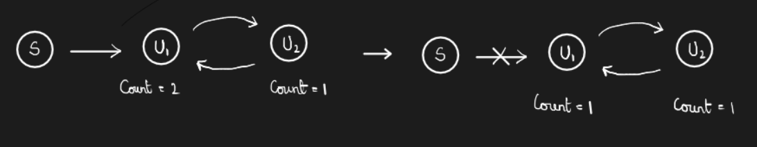
This problem does not occur in case of programming languages. The solution to this problem is TODO.
What about garbage collection when the program is huge? Is it efficient? Currently, many optimizations, like incremental garbage collection, have been implemented to prevent freezing of a program for garbage collection. Even after this, Java is not preferred for real-time applications. However, programmers prefer Java because of the ease of debugging and writing programs.
Roles
A role is a way to distinguish among various users as far as what these users can access/update in the database.
create a role <name>
grant <role> to <users>
There are a couple more features in authorization which can be looked up in the textbook.
We can also give authorization on views.
Other authorization features
-
references privilege to create foreign key
grant reference (dept_name) on department to Mariano -
transfer of privileges
grant select on department to Amit with grant option;
revoke select on department from Amit, Satoshi cascade;
revoke select on deparment from Amit, Satoshi restrict;
Lecture 8
18-01-22
~ Chapter 5: Advanced SQL
Programming languages with automatic garbage collection cannot clean the data in databases. That is, if you try using large databases, then your system may hang.
JDBC code
DriverManager.getConnection("jdbc:oracle:thin:@db_name") is used to connect to the database. We need to close the connection after the work since each connection is a process on the server, and the server can have limited number of processes. In Java we check the null value using wasNull() function (not intuitive).
Prepared statements are used to take inputs from the user without SQL injection. We can also extract metadata using JDBC.
SQL injection
The method where hackers insert SQL commands into the database using SQL queries. This problem is prevented by using prepared statements.
This lecture was cut-short, and hence has less notes.
Lecture 9
20-01-22
Functions and Procedures
Functions and procedures allow ‘business logic’ to be stored in the database and executed from SQL statements.
We can define a function using the following syntax
create function <name> (params)
	returns <datatype>
	begin
		...
	end
You can return scalars or relations. We can also define external language routines in other programming languages. These procedures can be more efficient than the ones defined in SQL. We can declare external language procedures and functions using the following.
create procedure <name>(in params, out params (?))
language <programming-language>
external name <file_path>
However, there are security issues with such routines. To deal with security problems, we can
- sandbox techniques - using a safe language like Java which cannot access/damage other parts of the database code.
- run external language functions/procedures in a separate process, with no access to the database process’ memory.
Triggers
When certain actions happen, we would like the database to react and do something as a response. A trigger is a statement that is executed automatically by the system as a side effect of a modification to the database. To design a trigger mechanism, we must specify the conditions under which the trigger is to be executed and the actions to be taken when the trigger executes. The syntax varies from database to database and the user must be wary of it.
The SQL:1999 syntax is
create trigger <name> after [update, insert, delete] of <relation> on <attributes>
referencing new row as nrow
referencing old row as orow
[for each row]
	...
If we do not want the trigger to be executed for every row update, then we can use statement level triggers. This ensures that the actions is executed for all rows affected by a transaction. We use for each instead of for each row and we reference tables instead of rows.
Triggers need not be used to update materialized views, logging, and many other typical use cases. Use of triggers is not encouraged as they have a risk of unintended execution.
Recursion in SQL
SQL:1999 permits recursive view definition. Why do we need recursion? For example, if we want to find which courses are a prerequisite (direct/indirect) for a specific course, we can use
with recursive rec_prereq(course_id, prereq_id) as (
	select course_id, prereq_id from prereq
	union
	select rec_prereq.course_id, prereq.prereq_id,
	from rec_prereq, prereq
	where rec_prereq.prereq_id = prereq.course_id
) select * from rec_prereq;
This example view, rec_prereq is called the transitive closure of the prereq relation. Recursive views make it possible to write queries, such as transitive closure queries, that cannot be written without recursion or iteration. The alternative to recursion is to write a procedure to iterate as many times as required.
The final result of recursion is called the fixed point of the recursive view. Recursive views are required to be monotonic. This is usually achieved using union without except and not in.
Advanced Aggregation Features
Ranking
Ranking is done in conjunction with an order by specification. Can we implement ranking with the knowledge we have currently? Yes, we can use count() to check how many tuples are ahead of the current tuple.
select *, (select count(*) from r as r2 where r2.t > r1.t) + 1 from r as r1
However, this is \(\mathcal O(n^2)\). Also, note that the above query implements sparse rank. Dense rank can be implemented using the unique keyword. Rank in SQL can be implemented using rank() over ([order by A desc]).
Ranking can be done within partitions within the dataset. This is done using partition by. The whole query is given by
select ID, dept_name, rank() over
	(partition by dept_name order by GPA desc)
from dept_grades
order by dept_name, dept_rank
Multiple rank clauses can occur in a single select clause! Ranking is done after applying group by clause/aggregation. Finally, if we want only the top few ranks, we can use limit. However, this method is restrictive as we can’t select top-n in each partition and it is inherently non-deterministic. This is because ties are broken arbitrarily. It is usually better to select directly using the rank attribute by embedding the relation in an outer query.
Ranking has other function such as
-
percent_rankgives percentile -
cume_distgives fraction -
row_number(non-deterministic)
SQL:1999 permits the user to specify nulls first or nulls last.
For a given constant \(n\), the function ntile(n) takes the tuples in each partition in the specified order, and divides them into \(n\) buckets with equal number of tuples.
Windowing
Here are the examples of window specifications
between rows unbounded preceding and current
rows nbounded preceding
range between 10 preceding and current row
range interval 10 day preceding
-- Given a relation transaction
-- where value is positive for a deposite and
-- negative for a withdrawal, find total balance
-- of each account after each transaction on it
select account_number, date_time,
	sum(value) over
		(partition by account_number
        order by date_time
        rows unbounded preceding)
   	as balance
from transaction
order by account_number, date_time
We can perform windowing within partitions.
Lecture 10
24-01-22
We will cover one last concept in SQL and then move on to ER models.
OLAP
OLAP stands for Online Analytical Processing. It allows interactive analysis of data, allowing data to be summarized and viewed in different ways in an online fashion. Data that can be modeled as dimension attributes and measure attributes are called multidimensional data. Measure attributes measure some value that can be aggregated upon. Dimension attributes define the dimension on which measure attributes are viewed.
Items are often represented using cross-tabulation (cross-tab), also referred to as a pivot table. The dimension attributes form the row and column headers. The measure attributes are mentioned in each individual cell. Similarly, we can create a data cube which is a multidimensional generalization of a cross-tab. We can represent cross-tabs using relations. These can be used in SQL with null representing the total aggregates (despite the confusion).
The cube operation in SQL computes the union of group by’s on every subset of the specified attributes. The function grouping() can be applied on an attribute to check if the null value represents ‘all’ or not. It returns 1 if the value is a null value representing all. The rollup construct generates union on every prefix of a specified list of attributes. It can be used to generate aggregates at multiple levels of a hierarchy.
OLAP Operations
- Pivoting - Changing the dimensions used in a cross-tab
- Slicing - Creating a cross-tab for fixed values only. Sometimes called dicing when values for multiple dimensions are fixed.
- Rollup - Moving from finer-granularity data to a coarser granularity.
- Drill down - Opposite of rollup.
Early OLAP systems precomputed all possible aggregates in order to provide online response. Since this is infeasible, it suffices to precompute some aggregates and compute others on demand from pre-computed aggregates.
~Chapter 6: Database Design using the ER Model
How do we design schemas for a database? Is there any systematic way? We shall study this in the following chapter. The entity-relationship model proves useful in modelling the data.
When we design a database, we initially characterize the data needs of the database users. Then, we choose a data model to translate the requirements into a conceptual schema. The conceptual schema is designed using the ER model, and the implementation can be done in different ways such as the relation model. We do this in the final step where we move from an abstract data model to the implementation in the database.
Why do we care about good design? A bad design can have redundancy - repeats information which might cause data inconsistency and incompleteness which might make certain aspects of the enterprise difficult or impossible to model.
ER Model
Entity is a thing or an object in the enterprise that is distinguishable from other objects. It is described by a set of attributes. A relationship is an association among several entities. These models are represented graphically using the ER diagram.
Entity sets
An entity set is a set of entities of the same type that share the same properties. For example, it can be a set of all persons (each of which is an entity). A subset of the attributes form a primary key of the entity set.
Entity sets can be represented graphically using rectangles and attributes listed inside it. The primary keys are underlined.
Relationship sets
A relationship set is a mathematical relation among \(n \geq 2\) entities, each taken from entity sets.
\[\{(e_1, e_2, \dots, e_n \vert e_1 \in E_1, e_2 \in E_2, \dots, e_n \in E_n\}\]where \((e_1, e_2, \dots, e_n)\) is a relationship. We draw a line between the related entities to represent relationships. Relationship sets are represented using diamonds.
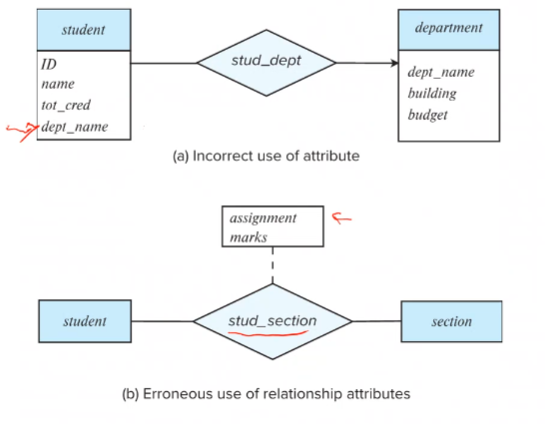
An attribute can also be associated with a relationship set. This is shown using a rectangle with the attribute name inside connected to the relationship set diamond with a dotted line.
Roles
The entity sets of a relationship need not be distinct. In such a case, we assign ‘roles’ to the entity sets.
Degree of a relationship set
The degree of a relationship set is defined as the number of entities associated with the relationship set. Most relationship sets are binary. We can’t represent all ternary relations as a set of binary relations.
There are no null values in the ER model. This becomes an issue in case of ternary relationships. Such problems are prevented in binary relationships. For example, think about the ER model of people and their parents. If someone has only one parent, then it is difficult to represent this using a ternary relationship between people, fathers and mothers. Instead, we could have two separate father and mother relationships. Binary relationships also provide the flexibility of mapping multiple entities to the same entity between two entity sets. While this is also possible in ternary relationships, we have more options in case of binary relationships.
Does ternary relationship convey more information than binary relationship in any case? Yes, that is why we can’t represent all ternary relations as a set of binary relations. For instance, think about the instructor, project and student mapping. There are many combinations possible here which can’t be covered using binary relationships.
Complex attributes
So far, we have considered atomic attributes in the relation model. The ER model does not impose any such requirement. We have simple and composite attributes. A composite attribute can be broken down into more attributes. For instance, we can have first and last name in name. We can have single-valued and multi-valued attributes. We can also have derived attributes. Multivalued attributes are represented inside curly braces {}.
Mapping cardinality constraints
A mapping cardinality can be one-to-one, one-to-many, many-to-one or many-to-many.
Lecture 11
25-01-22
We express cardinality constraints by drawing either a directed line \((\to)\), signifying ‘one’, or an undirected line \((-)\), signifying ‘many’, between the relationship set and the entity set.
Let us now see the notion of participation.
Total participation - every entity in the entity set participates in at least one relationship in the relationship set. This is indicated using a double line in the ER diagram.
Partial participation - some entities may not participate in any relationship in the relationship set.
We can represent more complex constraints using the following notation. A line may have an associated minimum and maximum cardinality, shown in the form ‘l..h’. A minimum value of 1 indicates total participation. A maximum value of 1 indicates that the entity participates in at most one relationship. A maximum value of * indicates no limit.
How do we represent cardinality constraints in Ternary relationships? We allow at most one arrow out of a ternary (or greater degree) relationship to indicate a cardinality constraint. For instance, consider a ternary relationship R between A, B and C with arrows to B, then it indicates that each entity in A is associated with at most one entity in B for an entity in C.
Now, if there is more than one arrow, the understanding is ambiguous. For example, consider the same setup from the previous example. If there are arrows to B and C, it could mean
- Each entity in A is associated with a unique entity from B and C, or
- Each pair of entities from (A, B) is associated with a unique C entity, and each pair (A, C) is associated with a unique entity in B.
Due to such ambiguities, more than one arrows are typically not used.
Primary key for Entity Sets
By definition, individual entities are distinct. From the database perspective, the differences are expressed in terms of their attributes. A key for an entity is a set of attributes that suffice to distinguish entities from each other.
Primary key for Relationship Sets
To distinguish among the various relationships of a relationship set we use the individual primary keys of the entities in the relationship set. That is, for a relationship set \(R\) involving entity sets \(E_1, E_2, \dots, E_n\), the primary key is given by the union of the primary keys of \(E_1, E_2, \dots, E_n\). If \(R\) is associated with any attributes, then the primary key includes those too. The choice of the primary key for a relationship set depends on the mapping cardinality of the relationship set.
Note. In one-to-many relationship sets, the primary key of the many side acts as the primary key of the relationship set.
Weak Entity Sets
Weak entity set is an entity set whose existence depends on some other entity set. For instance, consider the section and course entity set. We cannot have a section without a course - an existence dependency. What if we use a relationship set to represent this? This is sort of redundant as both section and course have the course ID as an attribute. Instead of doing this, we can say that section is a weak entity set identified by course.
In ER diagrams, a weak entity set is depicted via a double rectangle. We underline the discriminator of a weak entity set with a dashed line, and the relationship set connecting the weak entity set (using a double line) to the identifying strong entity set is depicted by a double diamond. The primary key of the strong entity set along with the discriminators of the weak entity set act as a primary key for the weak entity set.
Every weak entity set must be associated with an identifying entity set. The relationships associating the weak entity set with the identifying entity set is called the identifying relationship. Note that the relational schema we eventually create from the weak entity set will have the primary key of the identifying entity set.
Redundant Attributes
Sometimes we often include redundant attributes while associating two entity sets. For example, the attribute course_id was redundant in the entity set section. However, when converting back to tables, some attributes get reintroduced.
Reduction to Relation Schemas
Entity sets and relationship sets can be expressed uniformly as relation schemas that represent the content of the database. For each entity set and relationship set there is a unique schema that is assigned the name of the corresponding entity set or relationship set. Each schema has a number of columns which have unique names.
- A strong entity set reduces to a schema with the same attributes.
- A weak entity set becomes a table that includes a column for the primary key of the identifying strong entity set.
- Composite attributes are flattened out by creating separate attribute for each component attribute.
- A multivalued attribute \(M\) of an entity \(E\) is represented by a separate schema \(EM\). Schema \(EM\) has attributes corresponding to the primary key of \(E\) and an attribute corresponding to multivalued attribute \(M\).
- A many-to-many relationship set is represented as a schema with attributes for the primary keys of the two participating entity sets, and any descriptive attributes of the relationships set.
- Many-to-one and one-to-many relationship sets that are total on the many-side can be represented by adding an extra attribute to the ‘many’ side. If it were not total, null values would creep up. It is better to model such relationships as many-to-many relationships so that the model needn’t be changed when the cardinality of the relationship is changed in the future.
Extended ER Features
Specialization - Overlapping and Disjoint; Total and partial.
How do we represent this in the schema? Form a schema for the higher-level entity and for the lower-level entity set. Include the primary key of the higher level entity set and local attributes in that of the local one. However, the drawback of such a construction is that we need to access two relations (higher and then lower) to get information.
Generalization - Combine a number of entity sets that share the same features into a higher-level entity set.
Completeness constraint specifies whether or not an entity in the higher-level entity set must belong to at least on of the lower-level entity sets within a generalization (total and partial concept). Partial generalization is the default.
Aggregation can also be represented in the ER diagrams.
- To represent aggregation, create a schema containing - primary key of the aggregated relationship, primary key of the associated entity set, and any descriptive attributes.
I don’t understand aggregation
Design issues
Lecture 12
27-01-22
Binary vs. Non-Binary Relationships
We had discussed this previously in this section. In general, any non-binary relationship can be represented using binary relationships by creating an artificial entity set. We do this by replacing \(R\) between entity sets \(A, B, C\) by an entity set \(E\), and three relationship sets \(R_i\) relating \(E\) and \(i \in \{A, B, C\}\). We create an identifying attribute for E and add any attributes of \(R\) to \(E\). For each relationship \((a_i, b_i, c_i)\) in \(R\), we
- create a new entity \(e_i\) in the entity set \(E\)
- add \((e_i, j_i)\) to \(R_j\) for \(j \in \{A, B, C\}\)
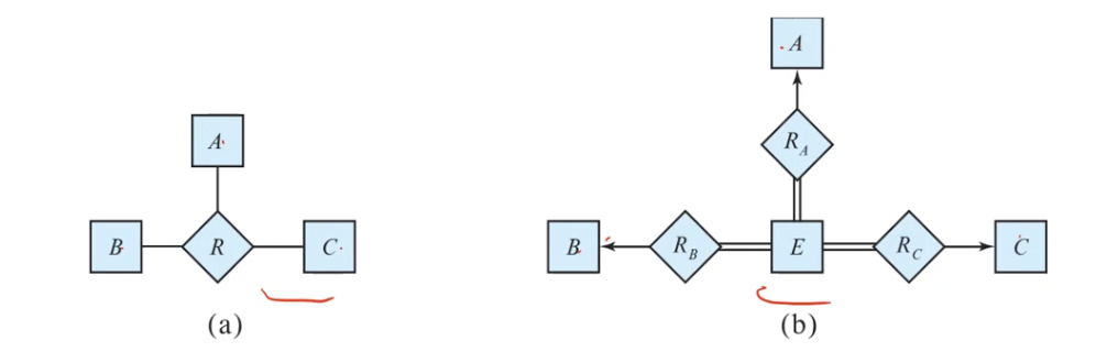
We also need to translate constraints (which may not be always possible). There may be instances in the translated schema that cannot correspond to any instance of \(R\). We can avoid creating an identifying attribute for \(E\) by making it a weak entity set identified by the three relationship sets.
ER Design Decisions
Important Points
- A weak entity set can be identified by multiple entity sets.
- A weak entity set can be identified by another weak entity set (indirect identification).
- In SQL, the value in a foreign key attribute can be null (the attribute of the relation having the fks constraint).
UML
The Unified Modeling Language has many components to graphically model different aspects of an entire software system. The ER diagram notation we studied was inspired from the UML notation.
~Chapter 7: Functional Dependencies
When programmers usually skip the design phase, they run into problems with their relational database. We shall briefly mention these problems and see the motivation for this chapter.
A good relational design does not have repetition of information, and no unnecessary null values. The only way to avoid the repetition of information is to decompose a relation to different schemas. However, all decompositions are not lossless.
Lecture 13
31-01-22
The term lossy decomposition does not imply loss of tuples but rather the loss of information (relation) among the tuples. How do we formalise this idea?
Lossless Decomposition - 1
Let \(R\) be a relations schema and let \(R_1\) and \(R_2\) form a decomposition of \(R = R_1 \cup R_2\). A decomposition if lossless if there is no loss of information by replacing \(R\) with the two relation schemas \(R_1, R_2\). That is,
\[\pi_{R_1}(r) \bowtie \pi_{R_2}(r) = r\]Note that this relations must hold for all instances to call the decomposition lossless. And, conversely a decomposition is lossy if
\[r \subset \pi_{R_1}(r) \bowtie \pi_{R_2}(r)\]We shall see the sufficient condition in a later section.
Normalization theory
We build the theory of functional/multivalued dependencies to decide whther a particular relation is in a “good” form.
Functional Dependencies
An instance of a relations that satisfies all such real-world constriants is called a legal instance of the relation. A functional dependency is a generalization of the notion of a key.
Let \(R\) be a relation schema and \(\alpha, \beta \subseteq R\). The functional dependency \(\alpha \to \beta\) holds on \(R\) iff for any legal relations \(r(R)\) whenever two tuples \(t_1, t_2\) of \(r\) agree on the attributes \(\alpha\), they also agree on the attributes \(\beta\). That is,
\[\alpha \to \beta \triangleq t_1[\alpha] = t_2[\alpha] \implies t_1[\beta] = t_1[\beta]\]Closure properties
If \(A \to B\) and \(B \to C\) Then \(A \to C\). The set of all functional dependencies logically implied by a functional dependency set \(F\) is the closure of \(F\) denoted by \(F^+\).
Keys and Functional Dependencies
\(K\) is a superket for relation schema \(R\) iff \(K \to R\). \(K\) is a candidate key for \(R\) iff
- \(K \to R\) and
- for no \(A \subset K\), \(A \to R\)
Functional dependencies allow us to express constraints that cannot be expressed using super keys.
Use of functional dependencies
We use functional dependencies to test relations to see if they are legal and to specify constraints on the set of legal relations.
Note. A specific instance of a relation schema may satisfy a functional dependency even if that particular functional dependency does not hold across all legal instances.
Lossless Decomposition - 2
A decomposition of \(R\) into \(R_1\) and \(R_2\) is lossless decomposition if at least one of the following dependecnies is in \(F^+\)
- \[R_1 \cap R_2 \to R_1\]
- \[R_1 \cap R_2 \to R_2\]
The above functional dependencies are a necessary condition only if all constraints are functional dependencies.
Dependency Preservation
Testing functional dependency constrinats each time the database is updated can be costly. If testing a functional dependency can be done by considering just one relation, then the cost of testing this constraint is low. A decomposition that makes it computaitonally hard to enforce functional dependencies is sat to be not dependency preserving.
Lecture 14
01-02-22
Boyce-Codd Normal Form
There are a few designs of relational schema which prevent redundancies and have preferable properties. One such design format is BCNF.
A relation schema \(R\) is in BCNF with respect to a set \(R\) of functional dependencies if for all functional dependencies in \(F^+\) of the form \(\alpha \to \beta\) where \(\alpha, \beta \subseteq R\), at least one of the following holds
- \(\alpha \to \beta\) is trivial (\(\beta \subseteq \alpha\))
- \(\alpha\) is a superkey for \(R\).
Let \(R\) Be a schema \(R\) That is not in BCNF. Let \(\alpha \to \beta\) Be the FD that causes a violation of BCNF. Then, to convert \(R\) to BCNF we decompose it to
- \[\alpha \cup \beta\]
- \[R - (\beta - \alpha)\]
Example. Consider the relation \(R= (A, B, C)\) with \(F \{A \to B, B \to C\}\). Suppose we have the following decompositions
- \[R_1 = (A, B), R_2 = (B, C)\]
This decompositions is lossless-join and also dependency preserving. Notice that it is dependency preserving even though we have the \(A \to C\) constraint. This is because \(A \to C\) is implied from the other two constraints.
- \[R = (A, B), R_2 = (A, C)\]
This decomposition is lossless but is not dependency preserving.
BCNF and Dependency Preservation
It is not always possible to achieve both BCNF and dependency preservation.
Third Normal Form
This form is useful when you are willing to allow a small amount of data redundancy in exchange for dependency preservation.
A relations \(R\) Is in third normal form (3NF) if for all \(\alpha \to \beta \in F^+\) at least one of the following holds
- \(\alpha \to \beta\) is trivial
- \(\alpha\) is a super key for \(R\)
- Each attribute \(A\) In \(\beta - \alpha\) is contained in a candidate key for \(R\).
There are 1NF and 2NF forms but they are not very important. If a relation is in BCNF, then it is in 3NF.
Redundancy in 3NF
Consider \(R\) which is in 3NF \(R = (J, K, L)\) and \(F = \{JK \to L, L \to K \}\). Then, we can have the following instance
| J | K | L |
|---|---|---|
| p1 | q1 | k1 |
| p2 | q1 | k1 |
| p3 | q1 | k1 |
| null | q2 | k2 |
3NF and Dependency Preservation
It is always possible to obtain a 3NF design without sacrificing losslessness or dependency preservation. However, we may have to use null values (like above) to represent some of the possible meaningful relationships among data items.
Goals of Normalisation
A “good” schema consists of lossless decompositions and preserved dependencies. We can use 3NF and BCNF (preferable) for such purpose.
There are database schemas in BCNF that do not seem to be sufficiently normalised. Multivalued dependencies, Insertion anomaly, …
Functional Dependency Theory
Closure of a set of functional dependencies
We can compute \(F^+\) from \(F\) by repeatedly applying Armstrong’s Axioms
- Reflexive rule - If \(\beta \subseteq \alpha\), then \(\alpha \to \beta\)
- Augmentation rule - If \(\alpha \to \beta\), then \(\gamma\alpha \to \gamma\beta\)
- Transitivity rule - If \(\alpha \to \beta\) and \(\beta \to \gamma\) then \(\alpha \to \gamma\)
It is trivial to see that these rules are sound. However, showing that these rules are complete is much more difficult.
Additional rules include (can be derived from above)-
- Union rule - If \(\alpha \to \beta\) and \(\alpha \to \gamma\), then \(\alpha \to \beta\gamma\)
- Decomposition rule - If \(\alpha \to \beta\gamma\), then \(\alpha \to \beta\)
- Pseudo-transitivity rule - If \(\alpha \to \beta\) and \(\gamma\beta \to \delta\), then \(\alpha \gamma \to \delta\)
Closure of Attribute Sets
Given a set of attributes \(\alpha\), define the closure of \(\alpha\) under \(F\) (denoted by \(\alpha^+\)) as the set of attributes that are functionally determined by \(\alpha\) under \(F\). We use the following procedure to compute the closure of A
result := A
while (change) do
	for each beta to gamma in F do
		begin
			if beta in result then result = result union gamma
    end
The time complexity of this algorithm is \(\mathcal O(n^3)\) where \(n\) is the number of attributes.
There are several uses of the attribute closure algorithm
- To test if \(\alpha\) is a superkey, we compute \(\alpha\) and check if it contains all attributes of the relation
- To check if a functional dependency \(\alpha \to \beta\) holds, see if \(\beta \subseteq \alpha^+\)
- For computing the closure of \(F\). For each \(\gamma \subseteq R\), we find \(\gamma\) and for each \(S \subset \gamma^+\), we output a functional dependency \(\gamma \to S\).
Canonical Cover
A Canonical cover of a functional dependency set \(F\) is the minimal set of functional dependencies such that its closure is \(F^+\).
An attribute of a functional dependency in \(F\) is extraneous if we can remove it without changing \(F^+\). Removing an attribute from the left side of a functional dependency will make it a stronger constraint.
Lecture 15
05-02-22
Extraneous attributes
Removing an attribute from the left side of a functional dependency makes it a stronger constraint. Attribute A is extraneous in \(\alpha\) if
- \[A \in \alpha\]
- \(F\) logically implies \((F - \{\alpha \to \beta\}) \cup \{(\alpha - A) \to \beta\}\)
To test this, consider \(\gamma = \alpha - \{A\}\). Check if \(\gamma \to \beta\) can be inferred from \(F\). We do this by computing \(\gamma^+\) using the dependencies in \(F\), and if it includes all attributes in \(\beta\) then \(A\) is extraneous in \(\alpha\).
On the other hand, removing an attribute from the right side of a functional dependency could make it a weaker constraint. Attribute A is extraneous in \(\beta\) if
- \[A \in \beta\]
-
The set of functional dependencies
\((F - \{\alpha \to \beta\}) \cup \{\alpha \to ( \beta - A)\}\) logically implies \(F\).
To test this, consider \(F’ = (F - \{\alpha \to \beta\}) \cup \{\alpha \to ( \beta - A)\}\) and check if \(\alpha^+\) contains A; if it does, then \(A\) is extraneous in \(\beta\).
Canonical Cover Revisited
A canonical cover for \(F\) is a set of dependencies \(F_c\) such that
- \(F\)(\(F_c\)) logically implies all dependencies in \(F_c\)(\(F\))
- No functional dependency in \(F_c\) contains an extraneous attribute
- Each left side of functional dependency in $$F_c$$ is unique
To compute a canonical cover for \(F\) do the following
Fc = F
repeat
	Use the union rule to replace any dependencies in Fc of the form
		alpha -> beta and alpha -> gamma with
    alpha -> beta gamma
	Find a functional dependency alpha to beta
	in Fc with an extraneous attribute
	in alpha or in beta
	Delete extraneous attribute if found
until Fc does not change
Dependency Preservation - 3
Let \(F_i\) be the set of dependencies \(F^+\) that include only the attribtues in \(R_i\). A decomposition is dependency preserving if \((F_1 \cup \dots \cup F_n)^+ = F^+\). However, we can’t use this definition to test for dependency preserving as it takes exponential time.
We test for dependency preservation in the following way. To check if a dependency \(\alpha \to \beta\) is preserved in a decomposition, apply the following test
result = alpha
repeat
	for each Ri in the decomposition
		t = (result cap Ri)^+ cap Ri
		result = result \cup t
until result does not change
If the result contains all attributes in \(\beta\), then the functional dependency \(\alpha \to \beta\) is preserved. This procedure takes polynomial time.
Testing for BCNF
To check if a non-trivial dependency \(\alpha \to \beta\) cause a violation of BCNF, compute \(\alpha^+\) and verify that it includes all attributes of \(R\). Another simpler method is to check only the dependencies in the given set \(F\) for violations of BCNF rather than checking all dependencies in \(F^+\). If none of the dependencies in \(F\) cause a violation, then none of the dependencies in \(F^+\) will cause a violation. Think.
However, the simplified test using only \(F\) is incorrect when testing a relation in a decomposition of \(R\). For example, consider \(R = (A, B, C, D, E)\), with \(F = \{ A \to B, BC \to D\}\) and the decomposition \(R_1 = (A, B), R_2 = (A, C, D, E)\). Now, neither of the dependencies in \(F\) contain only attributes from \((A, C, D, E)\) so we might be misled into thinking \(R_2\) satisfies BCNF.
Therefore, testing decomposition requires the restriction of \(R^+\) to that particular set of tables. If one wants to the use the original set of dependencies \(F\), then they must check that \(\alpha^+\) either includes no attributes of \(R_i - \alpha\) or includes all attributes of \(R_i\) for every set of attributes \(\alpha \subseteq R\). If a condition \(\alpha \to \beta \in F^+\) violates BCNF, then the dependency \(\alpha \to (\alpha^+ - \alpha) \cap R_i\) can be shown to hold on \(R_i\) and violate BCNF.
In conclusion, the BCNF decomposition algorithm is given by
result = R
done = false
compute F+
while (not done) do
	if (there is a schema Ri in result that is not in BCNF)
		let alpha to beta be a nontrivial functional dependency
      that holds on Ri such that alpha to Ri
      is not in F+
      and alpha cap beta is null
 		result = {(result - Ri),(Ri - beta),(alpha, beta)}
 	else done = true
Note that each \(R_i\) is in BCNF and decomposition is lossless-join.
3NF
The main drawback of BCNF is that is may not be dependency preserving. Through 3NF, we allow some redundancy to acquire dependency preserving along with lossless join.
To test for 3NF, we only have to check the FDs in \(F\) and not all the FDs in \(F^+\).We use attribute closure to check for each dependency \(\alpha \to \beta\), if \(\alpha\) is a super key. If \(\alpha\) is not a super key, we need to check if each attribute in \(\beta\) is contained in a candidate key of \(R\).
However, this test is shown to be NP-hard, but the decomposition into third normal form can be done in polynomial time.
Doesn’t decomposition imply testing? No, one relation can have many 3NF decompositions.
3NF Decomposition Algorithm
Let Fc be a canconical cover for F;
i = 0;
/* initial schema is empty */
for each FD alpha to beta in Fc do
	if none of the schemas Rj (j <= i) contains alpha beta
		then begin
			i = i + 1
			Ri = alpha beta
		end
/* Here, each of the FDs will be contained in one of the Rjs */
if none of the schemas Rj (j <= i) contains a candidate key for R
  then begin
    i = i + 1
    Ri = any candidate key for R
  end
/* Here, there is a relation contianing the candidate key of R */
/* Optionally remove redundant relations */
repeat
  if any schema Rj is contained in another schema Rk
    then delete Rj
      Rj = Ri;
      i = i - 1
  return (R1, ..., Ri)
Guaranteeing that the above set of relations are in 3NF is the easy part. However, proving that the decomposition is lossless is difficult.
Comparison of BCNF and 3NF
3NF has redundancy whereas BCNF may not be dependency preserving. The bigger problem is 3Nf allows certain function dependencies which are not super key dependencies. However, none of the SQL implementations today support such FDs.
Multivalued Dependencies
Let \(R\) be a relation schema and let \(\alpha, \beta \subseteq R\) . The multivalued dependency
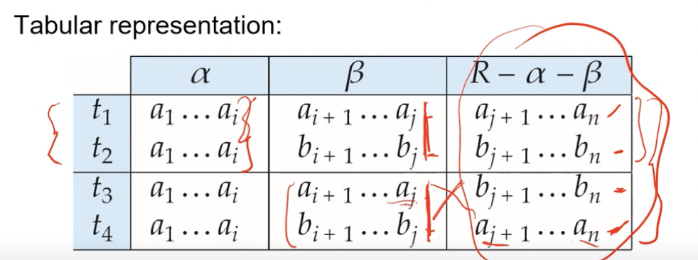
\[\alpha \to\to \beta\]holds on \(R\) if in any legal relation \(r(R)\), for all pairs for tuples \(t_1, t_2\) in \(r\) such that \(t_1[\alpha] = t_2[\alpha]\), there exists tuples \(t_3\) and \(t_4\) in \(r\) such that
\[t_1[\alpha] = t_2[\alpha] = t_3[\alpha] = t_4[\alpha] \\ t_3[\beta] = t_1[\beta] \\ t_3[R - \beta] = t_2[R - \beta] \\ t_4[\beta] = t_2[\beta] \\ t_4[R - \beta] = t_1[R - \beta]\]Intuitively, it means that the relationship between \(\alpha\) and \(\beta\) is independent of the remaining attributes in the relation. The tabular representation of these conditions is given by
The definition can also be mentioned in a more intuitive manner. Consider the attributes of \(R\) that are partitioned into 3 nonempty subsets \(W, Y, Z\). We say that \(Y \to\to Z\) iff for all possible relational instances \(r(R)\),
\[<y_1, z_1, w_1> \in r \text{ and } < y_1, z_2, w_2 > \in r \\ \implies \\ <y_1, z_1, w_2 > \in r \text{ and } <y_1, z_2, w_1 > \in r\]Important Points-
- If \(Y \to\to Z\) then \(Y \to\to W\)
- If \(Y \to Z\) then \(Y \to\to Z\)
why?
The closure \(D^+\) of \(D\) is the set of all functional and multivalued dependencies logically implied by \(D\). We are not covering the reasoning here.
Fourth Normal Form
A relation schema \(R\) is in 4NF rt a set \(D\) of functional and multivalued dependencies if for all multivalued dependencies in \(D^+\) in the form \(\alpha \to\to \beta\), where \(\alpha, \beta \subseteq R\), at least one of the following hold
- \(\alpha \to\to \beta\) is trivial
- \(\alpha\) is a super key for schema \(R\)
If a relation is in 4NF, then it is in BCNF. That is, 4NF is stronger than BCNF. Also, 4NF is the generalisation of BCNF for multivalued dependencies.
Restriction of MVDs
The restriction of \(D\) to \(R_i\) is the set \(D_i\) consisting of
- All functional dependencies in \(D^+\) that include only attributes of \(R_i\)
- All multivalued dependencies of the form \(\alpha \to \to (\beta \cap R_i)\) where \(\alpha \in R_i\) and \(\alpha \to\to \beta \in D^+\).
4NF Decomposition Algorithm
result = {R};
done = false;
compute D+
Let Di denote the restriction of D+ to Ri
while(not done)
	if (there is a schema Ri in result not in 4NF)
		let alpha to to beta be a nontrivial MVD that holds
		on Ri such that  alpha to Ri is not in Di and
		alpha cap beta is null
		result = {result - Ri, Ri - beta, (alpha, beta)}
	else done = true
This algorithm is very similar to that of BCNF decomposition.
Lecture 16
07-02-22
Further Normal Forms
Join dependencies generalise multivalued dependencies and lead to project-join normal form (PJNF) also known as 5NF. A class of even more general constraints leads to a normal form called domain-key normal form. There are hard to reason with and no set of sound and complete set of inference rules exist.
Overall Database Design Process
We have assumed \(R\) is given. In real life, we can get it based on applications through ER diagrams. However, one can consider \(R\) to be generated from a single relations containing all attributes that are of interest (called universal relation). Normalisation breaks this \(R\) into smaller relations.
Some aspects of database design are not caught by normalisation. For example, a crosstab, where values for on attribute become column names, is not captured by normalisation forms.
Modeling Temporal Data
Temporal data have an associated time interval during which the data is valid. A snapshot is the value of the data at a particular point in time. Adding a temporal component results in functional dependencies being invalidated because the attribute values vary over time. A temporal functional dependency \(X \xrightarrow{\tau} Y\) holds on schema \(R\) if the functional dependency \(X \to Y\) holds on all snapshots for all legal instances \(r(R)\).
In practice, database designers may add start and end time attributes to relations. SQL standard [start, end). In modern SQL, we can write
period for validtime (start, end)
primary key (course_id, validtime without overlaps)
~Chapter 8: Complex Data Types
Expected to read from the textbook.
- Semi-Structured Data
- Object Orientation
- Textual Data
- Spatial Data
Semi-Structured Data
Many applications require storage of complex data, whose schema changes often. The relational model’s requirement of atomic data types may be an overkill. JSON (JavaScript Object Notation) and XML (Extensible Markup Language) are widely used semi-structured data models.
Flexible schema
- Wide column representation allow each tuple to have a different set of attributes and can add new attributes at any time
- Sparse column representation has a fixed but large set of attributes but each tuple may store only a subset.
Multivalued data types
- Sets, multi-sets
- Key-value map
- Arrays
- Array database
JSON
It is a verbose data type widely used in data exchange today, There are efficient data storage variants like BSON
Knowledge Representation
Representation of human knowledge is a long-standing goal of AI. RDF: Resource Description Format is a simplified representation for facts as triples of the form (subject, predicate, object). For example, (India, Population, 1.7B) is one such form. This form has a natural graph representation. There is a query language called SparQL for this representation. Linked open data project aims to connect different knowledge graphs to allow queries to span databases.
To represent n-ary relationships, we can
- Create an artificial entity and link to each of the n entities
- Use quads instead of triples with context entity
Object Orientation
Object-relational data model provides richer type system with complex data types and object orientation. Applications are often written in OOP languages. However, the type system does not match relational type system and switching between imperative language and SQL is cumbersome.
To use object-orientation with databases, we could build an object-relational database, adding object-oriented features to a relational database. Otherwise, we could automatically convert data between OOP and relational model specified by object-relational mapping. Object-oriented database is another option that natively supports object-oriented data and direct access from OOP. The second method is widely used now.
Object-Relational Mapping
ORM systems allow
- specification of mapping between OOP objects and database tuples
- Automatic modification of database
- Interface to retrieve objects satisfying specified conditions
ORM systems can be used for websites but not for data-analytics applications!
Textual Data
Information retrieval basically refers to querying of unstructured data. Simple model of keyword queries consists of fetching all documents containing all the input keywords. More advanced models rank the relevance of documents.
Ranking using TF-IDF
Term is a keyword occurring in a document query. The term frequency \(TF(d, t)\) is the relevance of a term \(t\) to a document \(d\). It is defined by
\[TF(d, t) = \log( 1+ n(d, t)/n(d))\]where \(n(d, t)\) is the number of occurrences of term \(t\) in document \(d\) and \(n(d)\) is the number of terms in the document \(d\).
The inverse document frequency \(IDF(t)\) is given by
\[IDF(t) = 1/n(t)\]This is used to give importance to terms that are rare. Relevance of a document \(d\) to a set of terms \(Q\) can be defined as
\[r(d, Q) = \sum_{t \in Q} TF(d, t)*IDF(t)\]There are other definitions that take proximity of words into account and stop words are often ignored.
Lecture 17
08-02-22
The TF-IDF method in search engine was did not work out as web designers added repeated occurrences of words on their website to increase the relevance. There were plenty of shady things web designers could do in order to increase the page relevance. To prevent this problem, Google introduced the model of PageRank.
Ranking using Hyperlinks
Hyperlinks provide very important clues to importance. Google’s PageRank measures the popularity/importance based on hyperlinks to pages.
- Pages hyperlinked from many pages should have higher PageRank
- Pages hyperlinked from pages with higher PageRank should have higher PageRank
This model is formalised by a random walk model. Let \(T[i, j]\) be the probability that a random walker who is on page \(i\) will click on the link to page \(j\). Then, PageRank[j] for each page \(j\) is defined as
\[P[j] = \delta/N + (1 - \delta)*\sum_{i = 1}^n(T(i, j)*P(j))\]where \(N\) is the total number of pages and \(\delta\) is a constant usually set to \(0.15\). As the number of pages are really high, some sort of bootstrapping method (Monte Carlo simulation) is used to approximate the PageRank. PageRank also can be fooled using mutual link spams.
Retrieval Effectiveness
Measures of effectiveness
- Precision - what % of returned results are actually relevant.
- Recall - what percentage of relevant results were returned
Spatial Data
Not covered
~Chapter 9: Application Development
HTTP and Sessions
The HTTP protocol is connectionless. That is, once the server replied to a request, the server closes the connection with the client, and forgets all about the request. The motivation to this convention is that it reduces the load on the server. The problem however is authentication for every connection. Information services need session information to acquire user authentication only once per session. This problem is solved by cookies.
A cookie is a small piece of text containing identifying information
- sent by server to browser on first interaction to identify session
- sent by browser to the server that created the cookie on further interactions (part of the HTTP protocol)
- Server saved information about cookies it issued, and can use it when serving a request. E.g, authentication information, and user preferences
Cookies can be stored permanently or for a limited time.
Java Servlet defines an API for communication between the server and app to spawn threads that can work concurrently.
Web Services
Web services are basically URLs on which we make a request to obtain results.
Till HTML4, local storage was restricted to cookies. However, this was expanded to any data type in HTML5.
HTTP and HTTPS
The application server authenticates the user by the means of user credentials. What if a hacker scans all the packets going to the server to obtain a user’s credentials? So, HTTPS was developed to encrypt the data sent between the browser and the server. How is this encryption done? The server and the browser need to have a common key. Turns out, there are crypto techniques that can achieve the same.
What if someone creates a middleware that simulates a website a user uses? This is known as man in the middle attack. How do we know we are connected to the authentic website? The basic idea is to have a public key of the website and send data encrypted via this public key. Then, the website uses its own private key to decrypt the data. This conversion is reversible. As in, the website encrypts the data using its own private key which can be decoded by the user using the public key.
How do we get public keys for millions of websites out there? We use digital certificates. Let’s say we have a website’s public key and that website has the public key of the user (via their website). The website then encrypts the user’s public key using its private key to generate a digital certificate. This digital certificate can be advertised on the user’s website to allow other users to check the authenticity of the user’s website. Now, another user can obtain this certificate, decrypt it using the first website’s private key, and verify the authenticity of the user’s webpage. These verifications are maintained as a hierarchical structure to maintain digital certificates of millions of websites.
Cross Site Scripting
In cross site scripting, the user’s session for one website is used in another website to execute actions at the server of the first website. For example, suppose a bank’s website, when logged in, allows the user to transfer money by visiting the link xyz.com/?amt=1&to=123. If another website has a similar link (probably for displaying an image), then it can succeed in transferring the amount if the user is still logged into the bank. This vulnerability is called called cross-site scripting (XSS) or cross-site request forgery (XSRF/CSRF). XSRF tokens are a form of cookies that are used to check these cross-site attacks (CORS from Django).
Lecture 18
14-02-22
Application Level Authorisation
Current SQL standard does not allow fine-grained authorisation such as students seeing their own grades but not others. Fine grained (row-level) authorisation schemes such as Oracle Virtual Private Database (VPD) allows predicates to be added transparently to all SQL queries.
~Chapter 10: Big Data
Data grew in terms of volume (large amounts of data), velocity (higher rates of insertions) and variety (many types of data) in the recent times. This new generation of data is known as Big Data.
Transaction processing systems (ACID properties) and query processing systems needed to be made scalable.
Distributed File Systems
A distributed file system stores data across a large collection of machines, but provides a single file-system view. Files are replicated to handle hardware failure, and failures were to be detected and recovered from.
Hadoop File System Architecture
A single namespace is used for an entire cluster. Files are broken up into blocks (64 MB) and replicated on multiple DataNodes. A client finds the location of blocks from NameNode and accesses the data from DataNodes.
The key idea of this architecture is using large block sizes for the actual file data. This way, the metadata would be reduced and the NameNode can store the DataNodes info in a much more scalable manner.
Distributed file systems are good for millions of large files. However, distributed file systems have very high overheads and poor performance with billions of smaller tuples. Data coherency also needs to be ensured (write-once-read-many access model).
Sharding
It refers to partitioning data across multiple databases. Partitioning is usually done on some partitioning attributes known as partitioning keys or shard keys. The advantage to this is that it scales well and is easy to implement. However, it is not transparent (manually writing all routes and queries across multiple databases), removing load from an overloaded database is not easy, and there is a higher change of failure. Sharding is used extensively by banks today.
Key Value Storage Systems
These systems store large numbers of small sized records. Records are partitioned across multiple machines, and queries are routed by the system to appropriate machine. Also, the records are replicated across multiple machines to ensure availability. Key-value stores ensure that updates are applied to all replicas to ensure consistency.
Key-value stores may have
- uninterpreted bytes with an associated key
- Wide-column with associated key
- JSON
Document stores store semi-structured data, typically JSON. Key-value stores support put, get and delete. Some systems also support range queries on key values. Document stores also support queries on non-key attributes. Key value stores are not full database systems. They have no/limited support for transactional updates and applications must manage query processing on their own. These systems are therefore known as NoSQL systems.
Parallel and Distributed Databases
Replication to ensure availability. Consistency implemented using majority protocols. Network partitions involve a network can break into two or more parts, each with active systems that can’t talk to other parts. In presence of partitions, cannot guarantee both availability and consistency - Brewer’s CAP theorem. Traditional database systems choose consistency, and most web applications choose availability.
Lecture 19
15-02-22
MapReduce Paradigm
The goal here is to be able to run many queries/scripts across a large number of machines. Map and Reduce have similar functionalities as seen in Python. Programmers realised many operations can be reduced to a sequence of map and reduce actions (popular in functional programming).
Google formalised the notion of map-reduce for web-crawling and other web-development needs as map-reduce workers. This paradigm was used along with distributed file systems.
The default input for the map operations is a line.
map(k, v) -> list(k1, v1)
reduce(k1, list(v1)) -> v2
However, map-reduce code for database queries was large. So, the developers at Facebook came up with Hive which converts SQL queries to map-reduce queries.
Algebraic Operations
We shall study these as a part of Spark.
Lecture 20
17-02-22
Algebraic Operations in Spark
Resilient Distributed Dataset (RDD) abstraction is a collection of records that can be stored across multiple machines. RDDs can be created by applying algebraic operations on other RDDs. This is a generalisation to RA where the operators can be any piece of code. RDDs can be lazily computed when needed. As in, the tree is executed only on specific functions such as saveAsTextFile() or collect().
Spark makes use of Java Lambda expressions with the following syntax.
s -> ArrayasList(s.split(" ")).iterate()
RDDs in Spark can be typed in programs, but not dynamically.
Streaming Data
Streaming data refers to data that arrives in a continuous fashion in contrast to data-at-rest.
Approaches to querying streams-
- Windowing - Break up stream into windows and queries are run on windows.
- Continuous Queries - Queries written e.g. in SQL, output partial result based on stream seen so far; query results are updated continuously.
- Algebraic operators on streams - Operators are written in an imperative language.
- Pattern Matching - Complex Even Processing (CEP) systems. Queries specify patterns, system detects occurrences of patterns and triggers actions.
- Lambda architecture - Split the stream into two, one output goes to stream processing system and the other to a database for storage.
There are stream extensions to SQL - Tumbling window, Hopping window, Sliding window and Sessions windows.
Publish Subscribe Systems
Public-subscribe (pub-sub) systems provide convenient abstraction for processing streams. For example, Apache Kafka
Graph Databases
A graph data model can be seen as a generalisation of the ER model. Every entity can be seen as a node, and every binary relationship is an edge. Higher degree relationships can be expressed as multiple binary relationships.
Check out Neo4J. Query languages for graph databases make it easy for graph traversal.
Lecture 21
28-02-22
Parallel graph processing
Two popular approaches have been devised for parallel processing on very large graphs
- Map-reduce and algebraic frameworks
- Bulk synchronous processing (BSP)
Bulk Synchronous Processing
Each vertex of a graph has data associated with it. The vertices are partitioned across multiple machines, and state of the nodes are kept in-memory. Now, in each step (superstep)
- Nodes process received messages
- Update their state
- Send further messages or vote to halt
- Computation ends when all nodes vote to halt, and there are no pending messages
The method is synchronous as the computation is done in steps. However, this method is not fault tolerant as all the computations need to be recomputed in case of a failure. Checkpoints can be created for restoration.
~Chapter 11: Data Analytics
- Data Analytics - The processing of data to infer patterns, correlations, or models for prediction.
- Data often needs to be extracted from various source formats, transformed to a common schema, and loaded into the data warehouse. (ETL)
- Data mining extends techniques developed by ML onto large datasets
- A data warehouse is a repository of information gathered from multiple sources, stored under a unified schema at a single site. It also permits the study of historical trends. The common schema is optimised for querying and not transactions. The schema is most often denormalized (faster query time).
- Data in warehouses can be stored as fact tables or dimension tables. The attributes of fact tables can be usually viewed as measure attributes (aggregated upon) or dimension attributes (small ids that are foreign keys to dimension tables).
- A fact table branching out to multiple dimension schema is a star schema. A snowflake schema has multiple levels of dimension tables (can have multiple fact tables).
- A data lake refers to repositories which allow data to be stored in multiple formats without schema integration. Basically, data is just dumped for future use.
- Data warehouses often use column-oriented storage.
~Chapter 12: Physical Storage Systems
The performance of a database engine depends on the way data is stored underneath. The storage hierarchy typically used is as follows
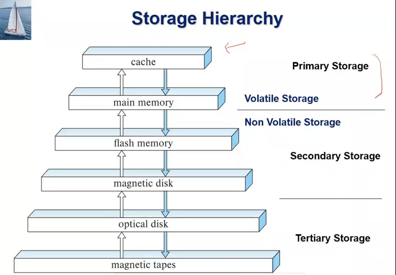
Tertiary storage is used for data archives in today’s world. Data is read as a cache-line from the main memory (lookahead sorta). Similarly, to account for even higher latency of the flash memory, we read one page at a time.
Storage Interfaces
The way we interface with the storage also has a great impact on the performance. We have the following standards
- SATA (Serial ATA) - Supports upto 6 Gbps (v3)
- SAS (Serial Attached SCSI) - Supports upto 12 Gbps (v3)
- NVMe (Non-Volatile Memory Express) works with PCIe connecters and gives upto 24 Gbps.
Lecture 22
03-03-22
A large number of disks are connected by a high-speed network to a number of servers in a Storage Area Network (SAN). The Network Attached Storage (NAS) provides a file system interface using a network file system protocol like FTP. SAN can be connected to multiple computers and gives a view of a local disk. It has fault tolerance and replication. A NAS pretends to be a file system unlike SAN.
Magnetic Disks
The surface of the platter is divided into 50k-100k circular tracks. Each track is divided into 500-1000 (on inner tracks) or 1000-2000 (on outer tracks) sectors. A cylinder is a stack of platters.
The performance of a disk is measured via its access time which involves seek time and rotational latency, I/O operations per second (IOPS), Mean/Annualized time to failure (MTTF) and data-transfer rate. We can tune the performance by changing parameters such as Disk block size and Sequential/Random access pattern. MTTF decreases as disk ages.
Note. Suppose the MTTF of a single disk is \(t\). How do we calculate the average failing time of a disk in a set of \(n\) disks? The probability that a disk fails in a given hour is \(1/t\). The probability that one of the disks in \(n\) fails is \(1 - (1 - 1/t)^n\). However, if \(t\) is large, it is simply \(n/t\). That is, on an average a disk fails in every \(t/n\) hours in a set of \(n\) disks.
In a random access pattern, every request requires a seek. This method results in lower transfer rates. Current disks allow up to 50-200 IOPS.
Flash storage
A NAND flash is widely used for storage in contrast to a NOR flash. A page can only be written once, and it must be erased to allow rewriting. Flash storage does page-at-a-time read. If we try for a byte read, then the control lines take up a lot of storage, and the capacity goes down.
A solid state disk uses standard block-oriented disk interfaces, but store data on multiple flash storage devices internally. We can use SSD using the SATA interface. An erase in flash storage happens in unit of erase block, and remapping of logical page addresses to physical page addresses avoids waiting for erase. The remapping is carried out by flash translation layer. After 100000 to 1000000 erases, the erase block becomes unreliable and cannot be use due to wear leveling.
A SLC tolerates about \(10^6\) erases. A QLC has 4 voltage levels (2 bits can be stored in 1 physical bit). These are much less tolerant to erases (about \(10^3\) erases). Wear leveling normalises the erases in a region of the flash storage by storing cold data in the part where a lot of erases have been done.
The performance of an SSD is measured through the data transfer rates. SSDs also support parallel reads. Hybrid disks combine small amount of flash cache with large magnetic disks.
Recently, Intel has come up with the 3D-XPoint memory technology which is shipped as Intel Optane. It allows lower latencies than flash SSDs.
RAID
Redundant Arrays of Independent Disks is a set of disk organization techniques that manage a large number of disks providing a view of a single disk. The idea is that some disk out of a set of N disks will fails much higher than the chance that a specific single disk will fail. We expect high capacity, high speed, and high reliability from this system.
In a way, we improve the reliability of the storage system using redundancy. For example, the simplest way to do this is mirroring (or shadowing) where we just duplicate all disks. The **mean time to data loss** depends on the mean time to failure and the mean time to repair. For example, if the MTTF is 100000 hours and the mean time to repair is 10 hours, then we get the mean time to data loss as \(500\times 10^6\) hours. How do we get this? The probability that one of the disk fails is \(2*10^{-5}\). Now, what is the probability that the other disk fails within the repair time? It is \(2* 10^{-4}\). Now, at this point we have data loss. Therefore, the mean time to data loss would be \(2.5 *10^8\) for one disk. As we have two disks, we get \(5 * 10^8\). Data loss occurs when both disks fail.
The two main goals of parallelism in a disk system are to load balance multiple small accesses to increase throughput and parallelise large accesses to reduce the response time. We do this via bit-level stripping or block-level striping. In block level striping, with n disks, block \(i\) of a file goes to disk to disk(\(i\%n\)) + 1. Now, requests for the same file can run in parallel increasing the transfer rate.
- RAID level 0 : Block-striping; non-redundant. Used in high-performance applications where data loss is not critical.
- RAID level 1: Mirrored disks with block striping. Popular for best write performance and applications such as storing log files in a database system.
RAID also parity blocks that stores the XOR of bits from the block of each disk. Parity block \(j\) stores XOR of bits from block \(j\) of each disk. This helps in recovery of data in case of a single disk failure (XOR the parity bit with the remaining blocks on various disks). Parity blocks are often spread across various disks for obvious reasons.
-
RAID level 5 - Block-interleaved Distributed Parity. This is nice but writes are slower. The cost of recovery is also high. Think.
-
RAID level 6 - It has a P + Q redundancy scheme where 2 error correction blocks are stored instead of a single parity block. Two parity blocks guard against multiple(2) disk failures.
There are other RAID levels which are not used in practice.
Lecture 23
07-03-22
Software RAID vs. Hardware RAID. Copies are written sequentially to guard against corruption in case of power failure. There are couple of hardware issues
- Latent sector failures - Data successfully written earlier gets damaged which can result in data loss even if only one disk fails.
- Data scrubbing - Continuous scans for latent failures, and recover from copy/parity.
- Hot swapping - Replacement of disk while the system is running without powering it down. This reduces the time to recovery, and some hardware RAID systems support this.
~Chapter 13: Data Storage Structures
File Organization
The database is stored as a collection of files. Each file is a sequence of records, and each record is a sequence of fields. We will assume the following
- Fixed record size
- Each file has records of one particular type only
- Different files are used for different relations
- Records are smaller than a disk block
Fixed length records
We store the records contiguously, and access a record based on the index and the offset. There might be fragmentation at the end of the block. How do we handle deleted records? We shall link all the free records on a free list.
Variable length records
Strings are typically variable sized. Each record has variable length attributes represented by fixed size (offset, length) with the actual data stored after all fixed length attributes. Null values are represented by null-value bitmap. How do we structure these records in a block?
Slotted Page Structure
A slotted page header contains -
- number of record entries
- end of free space in the block
- location and size of each record
The records are stored contiguously after the header. Disk pointers point to the header and not directly to the record.
Storing Large Objects
Records were assumed to be smaller than pages. Otherwise, we store the records as files. In Postgres, the large attribute is automatically broken up into smaller parts.
Organisation of Records in Files
Records can be stored as
- Heap - Record can be placed anywhere in the file where there is space. We maintain a hierarchical free space map of two levels usually.
- Sequential - Store records in sorted sequential order, based on the value of the search key of each record.
- B+ tree file organization
- Hashing
Some databases also support multi-table clustering file organisation that allows records of different relations to be stored in the same file.
Metadata and Partitioning
The data dictionary or system catalog stored metadata such as
- names of relations
- names, types and lengths of attributes of each relation
- names and definitions of views
- integrity constraints
Lecture 24
08-03-22
Partitioning
Table partitioning - Records in a relation can be partitioned into smalled relations that are stored separately - Horizontal partitioning. Store each attribute of a relation separately - vertical partitioning. Also known as columnar representation or column oriented storage. This is a good idea for data analytics but not for transaction processing. The benefits of this representation include
- Reduced IO if only some attributes are accessed
- Improved CPU cache performance
- Improved Compression
- Vector Processing on modern CPU architectures
The disadvantages are
- Tuple reconstruction is difficult
- Tuple deletion and updates are difficult
- Cost of decompression
Some databases support a hybrid model which has both row and column representation.
Note. ORC and Parquet use file formats with columnar storage inside file. These are log file formats.
Storage Access
Blocks are units of both storage allocation and data transfer. At the disk layer, a page is the physical unit. Buffer - The portion of the main memory to store copies of the disk blocks.
Buffer Manager
Pinned block - A memory block that is not allowed to be written back to the disk. A pin is done before reading/writing data from a block. An unpin done when read/write is complete. Multiple concurrent pin/unpin operations are possible. There are also shared and exclusive locks on buffer.
Buffer Replacement Policies
Most OS replace the block using the LRU strategy. However, this is not suitable in many database operations. Therefore, a database system can query plan to predict future references. There are toss-immediate and MRU strategies too.
~Chapter 14: Indexing
A search key is a set of attributes used to look up records in a file. An index file consists of records (called index entries) of the form \(search-key \mid pointer\). These files are usually much smaller than the original file. We have two basic kinds of indices
- Ordered indices - SEarch keys are stored in a sorted order
- Hash indices - search keys are distributed uniformly across “buckets” using a “hash function”.
Index Evaluation Metrics
- Access types supported by the indices. These include searching for records with a specified value or records falling in a specified range of values.
- Access time
- Insertion time
- Deletion time
- Space overhead
Ordered Indices
A clustering index in a sequentially ordered file, is the index whose search key specifies the sequential order of the file. It is also called as the primary index that is not to be confused with primary key. A secondary index/nonclustering is an index whose search key specifies an order different from the sequential order of the file.
An index sequential file is a sequential file ordered on a search key, with a clustering index on the search key.
Dense index Files
A dense index is an index for which there is a record in the index-file for every search-key value in the file. Also, every index-record made with a dense index need not be mapped to an index as we use the following structure.
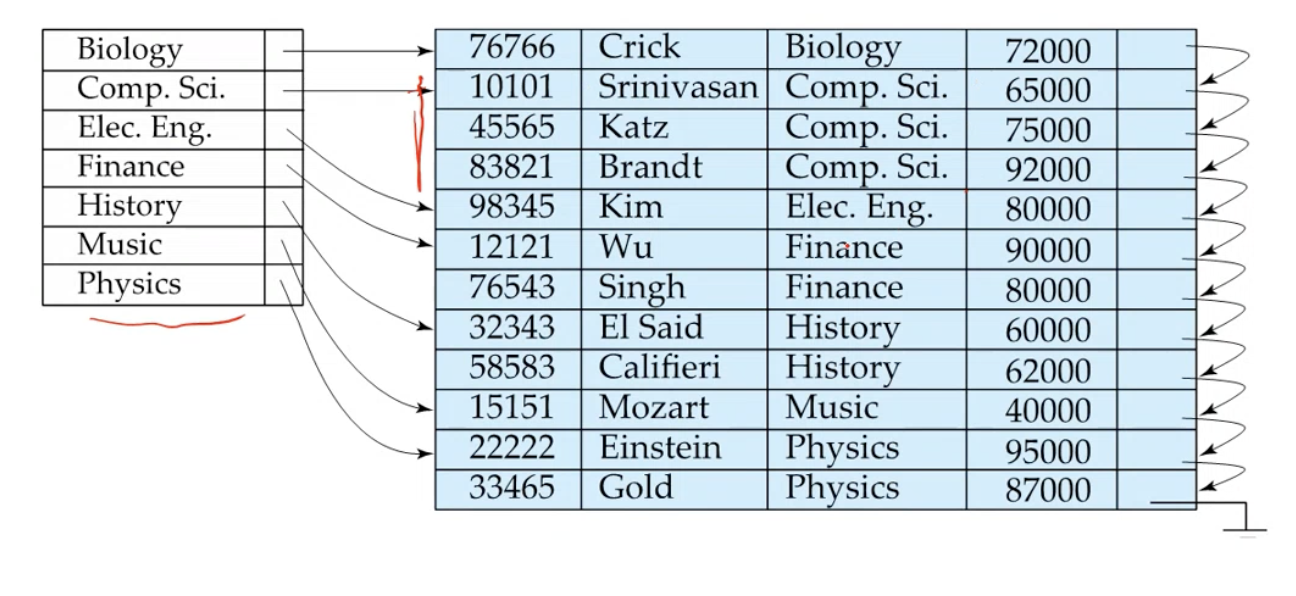
A sparse index on the other hand contains index records for only some search-key values. To locate a record with a search-key value \(K\), we first find an index record with largest search-key value \(< K\). Then, we search the file sequentially starting at the record to which the index record points. For unclustered index, we create a sparse index on top of a dense index (multilevel index).
Lecture 25
10-03-22
Sparse indices take less space and have less maintenance overhead in comparison to dense indices. However, they are generally slower than dense indices.
Note. Secondary indices have to be dense.
We use lexicographic ordering for composite search keys.
B\(^+\)-Tree
We will ignore duplicate keys for now. The number of children for every node lies within a certain specified range for that tree. In a \(B^+\)-Tree we have \(n\) pointers and \(n-1\) values separating them. A pointer between values \(a\) and \(b\) will point to values \(c\) that satisfy \(a \leq c < b\). It is not necessary for the internal nodes to be full.
Formally, a \(B^+\)-tree is a rotted tree satisfying the following properties
- All paths from the root to a leaf are of the same length.
- Each node that is not a root or a leaf has between \(\lceil{n/2}\rceil\) and \(n\) children.
- A lead node has between \(\lceil (n - 1)/2 \rceil\) and \(n - 1\) values.
- If a root is not a leaf, it has at least 2 children, and if a root is a lead, it can have between \(0\) and \(n - 1\) values.
A typical node looks like \(P_! \mid K_1 \mid \dots \mid K_{n - 1} \mid P_n\). Here \(K_i\) are the search-key values and \(P_i\) are pointers to children or records (buckets of records). Also, \(K_1 < \dots < K_{n - 1}\).
Leaf nodes
For \(i = 1, \dots, n - 1\), pointer \(P_i\) points to a file record with search-key value \(K_i\).
Pointers help us keep the nodes logically close but they need not be physically close. The non-lead levels of the \(B^+\) tree form a hierarchy of sparse indices. The level below root has at least \(2* \lceil n/2 \rceil\) values, the next level has \(2* \lceil n/2 \rceil* \lceil n/2 \rceil\), and so on. So if there are \(K\) search key values in the file, the tree height is no more than \(\lceil \log_{\lceil n/1 \rceil} K\rceil\).
Queries on \(B^+\)-trees
Range queries finds all records with search key values in a given range. These are implemented as iterators.
To handle non-unique keys, create a composite key that indexes into the duplicate values. Search for an index can be implemented as a range query. If the index is clustering, then all accesses are sequential. However, if the index if non-clustering, each record access may need an I/O operation.
Insertion on \(B^+\)-trees
Insertion is easy when the nodes are not full. However, when nodes are full, we would have to split the nodes. We split a node through the parent, by adding a splitting value in the parent node. We do this recursively, and if the root gets full, we create a new root. We insert from leaves because the leaves hold the pointers to records.
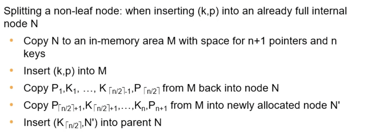
The above image gives the formal algorithm.
Deletion on \(B^+\)-trees
We need to ensure that there are at least a minimum number of values in each node. The complexity of the updates is of the order \(\mathcal O( \log_{\lceil n/2 \rceil}K)\). The height of the tree decreases when a node has very few children. Note that a deleted value can still appear as a separator in the tree after the deletion. Also, the average node occupancy depends on the insertion order (2/3rds with random and 1/2 with insertion in sorted order).
Lecture 26
14-03-22
If we allow non-unique keys, we can store a key with multiple pointers. However, the complexity comes in terms of deletion. Worst case complexity may be linear.
\(B^+\)-Tree file Organisation
Leaf nodes in a \(B^+\) tree file organisation store records, instead of pointers. As records are larger than pointers, the maximum number of records that can be stored in a lead node is less than the number of pointers in a non-leaf node. To improve space utilisation, we can involve more sibling nodes in redistribution during splits and merges. Involving 2 siblings in redistribution results in each node having at least \(\lfloor 2n/3 \rfloor\) entries.
Record relocation and secondary indices - If a record moves, all secondary indices that store record pointers have to be updated. Therefore, node splits in \(B^+\) tree file organisation become very expensive. The solution to this is use a search key of the \(B^+\) tree file organisation instead o record pointer in a secondary index. For example, consider students database sorted using roll numbers with names as a secondary index. If the records move, we would need to update all the “name” index pointers. So what we do is, make the “name” index pointers point to the “roll number” index pointers instead of the records directly. Since “roll number” is a clustered index, no relocation of secondary indices is required.
Indexing Strings
How do we use variable length strings as keys? We use prefix compression along with variable fanout (?). In the internal nodes, we can use simplified separators.
Bulk Loading and Bottom-Up Build
Inserting entries one-at-a-time into a \(B^+\)-tree requires \(\geq\) 1 I/O per entry assuming leaves don’t fit in the memory.
- Sort entries first, and insert in a sorted order. This will have much improved I/O performance.
- Build a \(B^+\)tree bottom-up. AS before sort the entries, and then create tree layer-by-layer starting with the leaf level.
However, the above two methods expect a bulk insertion. What do we do if we have a sudden burst of inserts? We will look at alternatives later.
B-Tree Index Files
Similar to \(B^+\)-tree but B-tree allows search-key values to appear only once and eliminates redundant storage of search keys. The pointers to the records are stored in the internal nodes too! The problem with this approach is that the tree becomes taller. There is minimal advantage too.
Indexing on flash has a few issues, as writes are no in-place and it eventually requires a more expensive erase.
A key idea is to use large node size to optimise disk access, but structure data within a node using a tree with small node size, instead of using an array for faster cache access (so that all nodes fit inside a single cache line).
Hashing
Handling bucket overflows
Overflow chaining - The overflow buckets of a given bucket are chained together in a linked list. The above scheme is called closed addressing or open/closed hashing.
Overflow can happen due to insufficient buckets or skewness in the data.
Hashing is not used widely on disks but is used in-memory.
Covering indices - Attributes that are added to index to prevent the control from fetching the entire record.
Some databases allow creation of indices on foreign keys.
Indices over tuples can be problematic for a few queries due to lexicographic ordering.
Lecture 27
15-03-22
Write Optimised Indices
Performance of \(B^+\) trees can be poor for write intensive workloads. This is because we require one I/O per leaf, assuming all internal nodes are in memory. There are two approaches to reducing cost of writes
- Log-structured merge tree
- Buffer tree
Log Structured Merge (LSM) Tree
Consider only insert queries for now. Records are first inserted into in-memory L0 tree. When the in-memory tree is full, we move the records to the disk in the L1 tree. \(B^+\)-tree is constructed using bottom-up by merging the existing L1 tree with records from L0 tree. The goal is to minimise random I/O.
The benefits are that inserts are done using sequential I/O operations and the leaves are full avoiding space wastage. The drawbacks are that queries have to search multiple trees and the entire context of each level is copied multiple times. Bloom filters avoid lookups in most trees. The idea is to use hash functions and bitmaps.
How about deletes? They will now incur a lot of I/O. We do a logical delete by inserting a new delete entry. Updates are handled as inserts followed by deletes.
LSM trees were introduced for disk-based indices. These are useful to minimise erases with flash-based indices.
Buffer Tree
Each internal node of \(B^+\)-tree has a buffer to store inserts. The inserts are moved to lower levels when the buffer is full. With a large buffer, many records are moved to lower level at each time. Therefore, per record I/O decreases.
The benefits are less overhead on queries, and it can be used with any tree index structure. However, they have more random I/O than LSM trees.
Spatial and Temporal Indices
A k-d tree is a structure used for indexing multiple dimensions. Each level of k-d tree partitions the space into two, and we cycle through the dimensions at each level. Range queries do not have \(\log\) complexity bounds in this index structure.
Queries can mix spatial (contains, overlaps) and non-spatial conditions.
The k-d-B tree extends the k-d tree to allow multiple child nodes for each internal node. This is well suited for secondary storage.
Each node in a quadtree is associated with a rectangular region of space. Similarly, we can cut across more dimensions in each level.
R-tree
The motivation behind this structure was to store objects in the spatial domain in a single leaf. We try to create minimally overlapping bounding boxes for all the objects and create a structure similar to a \(B^+\)-tree. Multiple paths may need to be searched, but the performance is good in practice.
Suppose we want to insert a new object that overlaps with many bounding boxes. We choose the box which overlaps the least, or the box which has the lowest change in size on the addition. Now, insertion is done via the clustering algorithm. The clustering is also done via some heuristics such as minimum overlap of bounding boxes. Greedy heuristics are often used.
Lecture 28
17-03-22
Indexing Temporal Data
A time interval has a start and an end time. A query may ask for all tuples that are valid at a point in time or during a time interval. We can use a spatial index called an R-tree for indexing.
~Chapter 15: Query Processing
Database engines often apply optimisations based on statistics over data which are approximate. An annotated expression specifying a detailed execution strategy is called an evaluation plan.
Query optimisation chooses an evaluation plan with the lowest cost (a metric based on approximated statistics).
Measures of Query Cost
Many factors contribute to time cost such as disk access, CPU, and network communication. Cost can be measured on response time or total resource consumption. As estimating the time is more difficult, we often resort to resource consumption for optimisation. This metric is also useful is shared databases. For our purposes, we will just consider costs related to I/O time.
Now, the disk cost is estimated as the sum of average seeks, blocks read, and blocks written. For simplicity we just use the number of block transfers from disk and the number of seeks. Then, we get \(b \times t_T + S\times t_S\). On a high end magnetic disk, \(t_S = 4ms, t_T = 0.1ms\) and on a SSD, \(t_S = 20-90\mu s, t_T = 2-10 \mu s\) for 4KB blocks.
We assume no data is available in the buffer.
Selection Operation
A1- Linear Search - Assume that file is stored sequentially.
cost = b/2*t_T + 1*t_S
We do not consider binary search as it requires a lot more (random) accesses and access time is high in disks.
Selection using Indices
A2 - Clustering index, Equality on key - Retrieve a single record that satisfied the corresponding equality condition.
cost = (h_i + 1)*(t_T + t_S)
Here, h_i is the height of the index (in \(B^+\)-tree?), and since we are doing random I/O for each case, we need to add both seek and transfer time.
A3-Clustering index, equality on non-key - Retrieve multiple records. Records will be on consecutive blocks. Let \(b\) be the number of blocks containing matching records.
cost = h_i*(t_T + t_S) + t_S + t_T*b
A4-Secondary index, equality on key/non-key
If the search-key is a candidate key, then
cost = (h_i + 1)*(t_T + t_S)
Why?
Otherwise, each of n matching records may b on a different block
cost = (h_i + n)*(t_T + t_S)
It might be cheaper to scan the whole relation as sequential access is easier than random I/O.
A5-Clustering index, comparison
cost = linear_cost for <
		 = index_equality_cost + linear_cost
A6-Non-clustering index, comparison
cost = cost + cost_records (I/O)
The difference between clustering and non-clustering indices is that we would have to fetch records in case of non-clustering indices in order to read the non-clustering index attribute. This is not the case in case of a clustering index.
Let me write my understanding of all this
Indices are just files with pointers. Basically, scanning through indices is faster than scanning through a sequence of entire records, so we use indices. Instead of storing indices sequentially, we use \(B^+\) trees so that its faster. We can’t do this with records directly because records are big and they may not reside in a single file (I think).
Now, clustering indices are indices whose order is same as the order of the records. So, once we fetch a record for an index, all records corresponding to the next indices will be in a sequence. Therefore, we won’t have additional seek time.
However, this is not the case for non-clustering indices. If we want records corresponding to the next indices of the current index, we’d have additional seek time as the records may lie in different blocks.
Implementation of Complex Selections
How do we implement conjunctions? If all the attributes in the conjunction are indexed, then it is straightforward. We will just take the intersection of all results. Otherwise, test all the other conditions after fetching the records into the memory buffer.
Also, as we discussed before, we can use a composite index.
Disjunctions are a slightly different. If we have all indexed attributes, we just take the union. Otherwise, we just have to do a linear scan. Linear scan is also the best way in most cases for negation.
Bitmap Index Scan
We have seen that index scans are useful when less number of records match in the case of secondary indices. If more records match, we should prefer a linear scan. How do we decide the method beforehand? The bitmap index scan algorithm is used in PostgreSQL.
We create a bitmap in memory with a bit for each page in the relation. A record ID is just the page ID and the entry number. We initially do an index scan to find the relevant pages, and mark these pages as 1 in the bitmap. After doing this, we just do a linear scan fetching only pages with bit set to 1.
How is the performance better? It is same as index scan when only a few bits are set, and it is same as a linear scan when most bits are set. Random I/O is avoided in both cases.
Sorting
For relations that fit in memory, we can use quicksort. Otherwise, we use external sort merge.
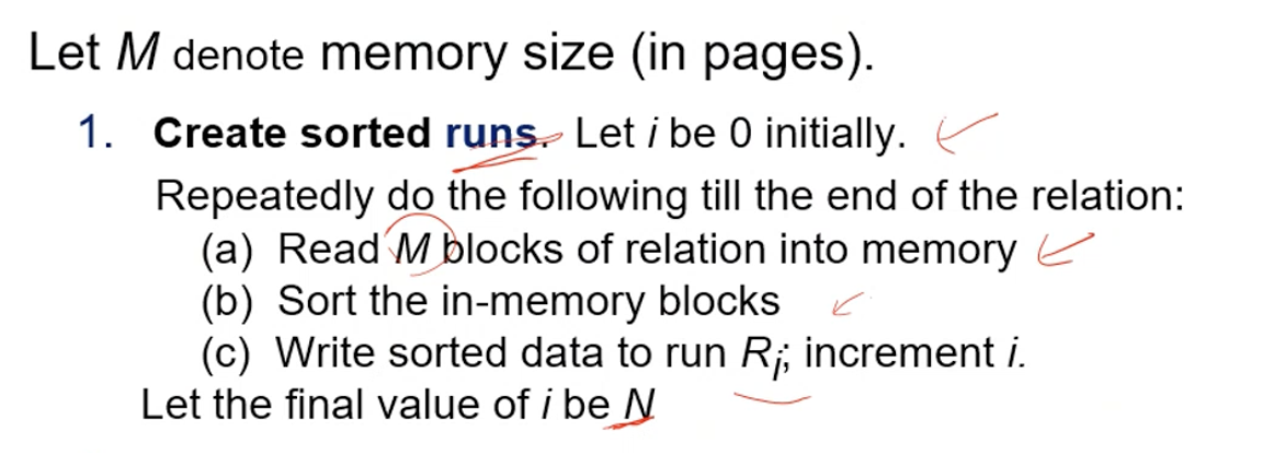
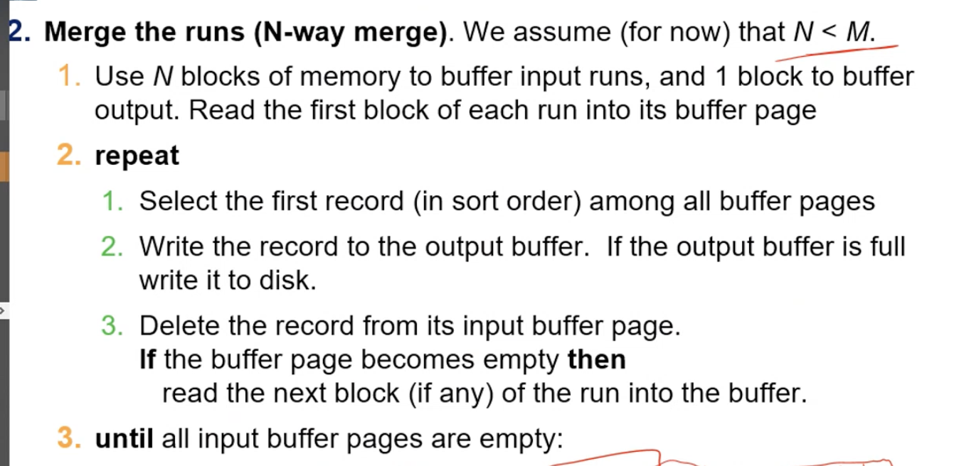
Lecture 29
21-03-22
Join Operation
Nested Loop Join
Requires no indices and can be used with any kind of join condition. It is very expensive though, as it is quadratic in nature. Most joins can be done in linear time in one of the relations, as most joins are foreign key joins. In the worst case, there would memory enough to hold only one block of each relation. The estimated cost then is, n_r*b_s + b_r block transfers and n_r + b_r seeks.
Block Nested-Loop Join
We first do block matching and then tuple matching. Asymptotically, this looks same as the above method but it decreases the I/O cost as the number of seeks come down.
Indexed Nested-Loop Join
An index is useful in equi-join or natural join. For each tuple \(t_r\) in the outer relation \(r\), we use the index to look up tuples in \(s\) satisfy the join condition with tuple \(t_r\). In the worst case, the buffer has space for only one page of \(r\), and for each tuple in \(r\), we perform an index lookup on \(s\). Therefore, the cost of the join is b_r(t_T + t_S) + n_r*C, where \(c\) is the cost of traversing index and fetching all matching \(s\) tuples for one tuple of \(r\). The second term is the dominating term. We should use the fewer tuples relations as the outer relation.
Merge Join
Sort both relations on their join attribute, and merge the sorted relations. Cost is (b_r + b_s)*t_T + (ceil(b_r/b_b) + ceil(b_S/b_b))*t_S along with the cost of sorting.
Hybrid merge-join - If one relation is sorted, an the other has a secondary \(B^+\)-tree on the join attribute, then we can merge the sorted relation with the leaf entries of the \(B^+\)-tree. Then we sort the result on the addresses of the unsorted relation’s tuples. Finally, we scan the unsorted relation in physical address order and merge with the previous result, to replace addresses by actual tuples.
Hash Join
The goal in the previous methods was to simplify the relations so that they fit in the memory. Along with this, we can also parallelise our tasks.
In this method, we hash on the join attributes and then merge each of the partitions. It is applicable for equi-joins and natural joins.
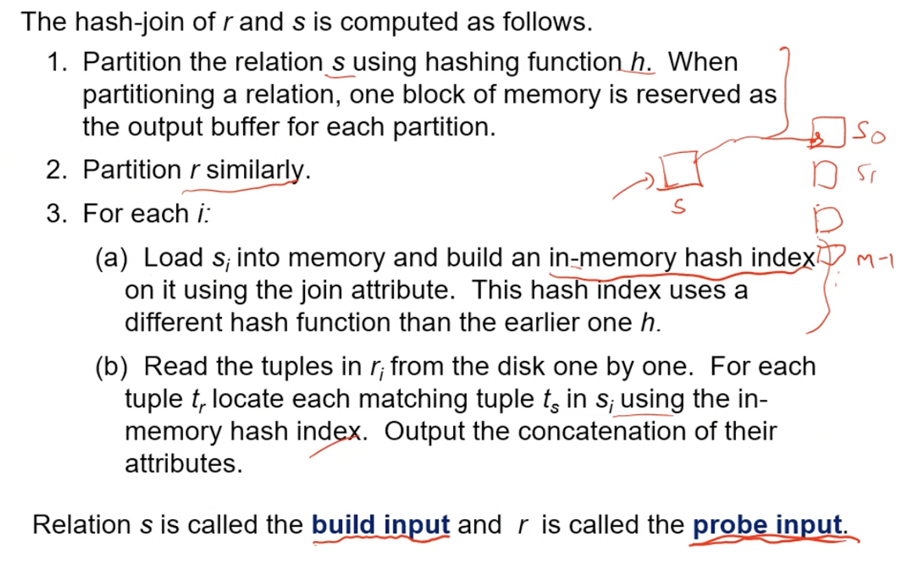
The value \(n\) and the hash function \(h\) are chosen such that each \(s_i\) fits in the memory. Typically, \(n\) is chosen as \(\lceil b_s/M \rceil *f\) where \(f\) is a fudge factor. The probe relation need not fit in memory. We use recursive partitioning if number of partitions is greater than number of pages in the memory.
Overflow resolution can be done in the build phase. Partition \(s_i\) is further partitioned using a different hash function. Overflow avoidance performs partitioning carefully to avoid overflows during the build phase. Both methods fail with a high number of duplicates.
Cost of hash join is (3(b_r + b_s) + 4n_h)*t_T + 2t_T(ceil(b_r/b_b) + ceil(b_s/b_b)). Recursive partitioning adds a factor of \(\log_{\lfloor M/bb\rfloor - 1}(b_s/M)\). If the entire build can be kept in the memory, then no partitioning is required and cost estimate goes down to \(b_r + b_s\).
Can we not build an entire index on \(s\) instead of hash join? Building an on-disk index is very expensive on disk. Indices have to be maintained which is an overhead.
Hybrid Hash-join keeps the first partition of the build relation in memory. This method is most useful when \(M \gg \sqrt b_s\).
Complex Joins
Similar methods to that of selection can be used here. That is conjunction of \(n\) conditions requires intersections of the result of \(n\) joins. In disjunction, we take the union of the join results. This method works for sets but not for multi-sets! For multi-sets, we can make sets out of the records.
Joins on Spatial Data
There is no simple sort order for spatial joins. Indexed nested loops join with spatial indices such as R-trees, quad-trees and k-d-B-trees. Nearest neighbour joins can be done with tiling.
Other operations
Duplicate elimination can be implemented via hashing or sorting. An optimisation is to delete duplicates during run generation as well as at intermediate merge steps. Projection can be done by performing projection on each tuple. Aggregation can implemented similar to duplicate elimination. Sorting and hashing can be used to bring tuples in the same group together, and then the aggregate functions can be applied on each group.
Lecture 30
22-03-22
Set Operations
These are fairly straightforward using merge-join after sorting or hash-join.
Outer Join
During merging, for every tuple \(t_r\) from \(r\) that do not match any tuple in \(s\), output \(t_r\) padded with nulls.
Evaluation of Expressions
We have two method to evaluate an entire expression tree
- Materialisation - Generate results of an expression whose inputs are relations or are already computed, materialize (store) it on disk
- Pipelining - Pass on tuples to parent operations even as an operation is being executed
Materialisation
We evaluate one operation at a time, and store each temporary result on the disk. this method is always applicable, but the cost is high. The overall cost is the sum of costs of individual operations and the cost of writing intermediate results to the disk.
Double buffering - Use two output buffers for each operation, when one is full write it to disk while the other is getting filled.
Pipelining
We evaluate several operations simultaneously, passing the results of one operation on to the next. However, this is not always possible in case of aggregation, sorts and hash-joins. It is executed in two ways -
- Demand driven - In lazy evaluation, the system repeatedly requests next tuple from the top level operation. The operation has to maintain states. Pull model.
- Producer driven - In eager pipelining the operators produce tuples eagerly and pass them up to their parents. Push model.
Blocking Operations
They cannot generate any output until all the input is consumed. For example, sorting, aggregation, etc. They often have two sub-operations, and we can treat them as separate operations. All operations in a pipeline stage run concurrently.
Query Processing in Memory
In early days, memory was the bottleneck. So, engineers had to reduce the I/O. Query was compiled to machine code, and compilation usually avoids many overheads of interpretations to speed up query processing. This was often done via generation of Java byte code with JIT compilation. Column oriented storage was preferred as it allowed vector operations, and cache conscious algorithms were used.
Lecture 31
24-03-22
Cache conscious algorithms
The goal is to minimise the cache misses.
- Sorting - We can use runs that are as large as L3 cache to avoid cache misses during sorting of a run. Then merge runs as usual in merge sort.
- Hash-join - We first create partitions such that build + probe partitions fit in memory. Then, we sub partition further such that sub partition and index fit in L3 cache. This speeds up probe phase.
- Lay out attributes of tuples to maximise cache usage. Store often accessed attributes adjacent to each other.
- Use multiple threads for parallel query processing. Cache miss leads to stall of one thread, but others can proceed.
~Chapter 16: Query Optimisation
As we have seen before, there are multiple ways to evaluate a given query. The cost difference can be magnanimous in some cases. A plan is evaluated on cost formulae, statistical information and statistical estimation of intermediate results. Most databases support explain <query> that gives the details of the evaluation plan.
Generating Equivalent Expressions
Two queries are equivalent in the (multi)set version if both of them generate the same (multi)set of tuples on every legal database instance. Note that we ignore the order of tuples in relational algebra.
-
Conjunctive selection operations can be deconstructed into a sequence of individual selections
\[\sigma_{\theta_1 \land \theta_2}(E) \equiv \sigma_{\theta_1} (\sigma_{\theta_2}(E))\] -
Selection operations are commutative
\[\sigma_{\theta_1} (\sigma_{\theta_2}(E)) \equiv \sigma_{\theta_2} (\sigma_{\theta_1}(E))\] -
Only the last in a sequence of project operations is needed, the others can be omitted.
\[\Pi_{L_1}(\dots(\Pi_{L_n}(E))\dots) \equiv \Pi_{L_1}(E)\] -
Selections can be combined with Cartesian products and theta joins.
\[\begin{align} \sigma_{\theta}(E_1 \times E_2) &\equiv E_1 \bowtie_\theta E_2 \\ \sigma_{\theta_1}(E_1 \bowtie_{\theta_2} E_2) & \equiv E_1 \bowtie_{\theta_1 \land \theta_2} E_2 \end{align}\] -
Theta-join and natural joins operations are commutative as well as associative. However, order will not be the same in SQL.
sc \((E_1 \bowtie_{\theta_1} E_2)\bowtie_{\theta_2 \land \theta_3} E_3 \equiv(E_1 \bowtie_{\theta_1 \land \theta_3} E_2)\bowtie_{\theta_2 } E_3\)
where \(\theta_2\) contains attributes only from \(E_2\) and \(E_3\).
- \[\sigma_{\theta_1 \land \theta_2} (E_1 \bowtie_\theta E_2) \equiv (\sigma_{\theta_1}(E_1)) \bowtie_\theta (\sigma_{\theta_2}(E_2))\]
-
Projection distributes over join. Throw out useless attributes before joining.
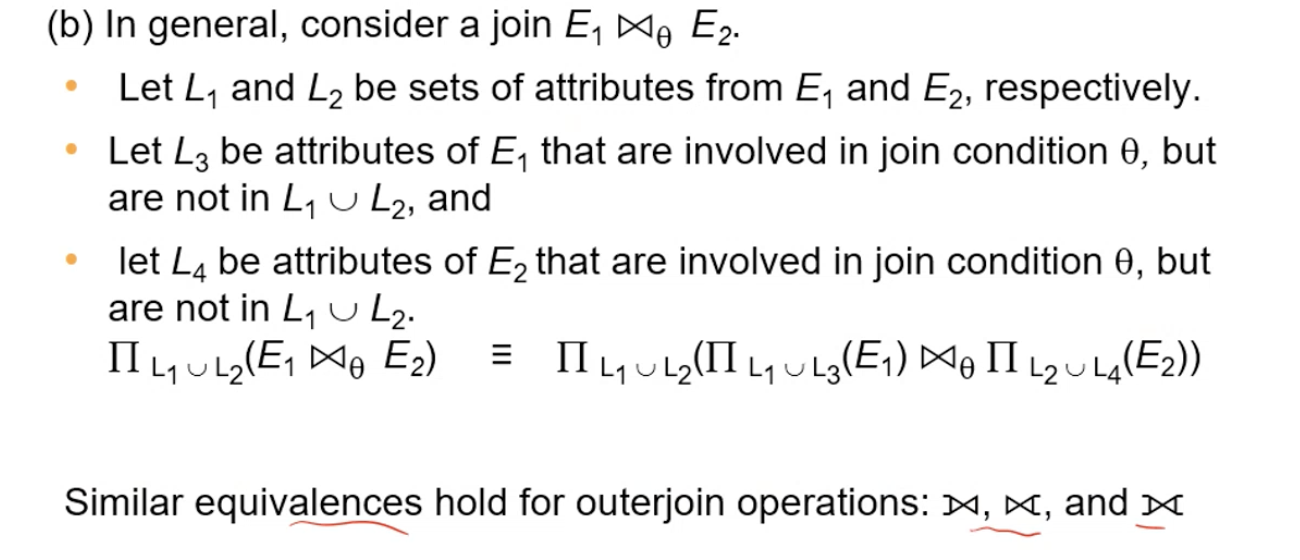
-
We also have the usual set operations equivalences. Selection operation distributes over \(\cup, \cap, -\).
-
We can also come up with rules involving left outer join (⟖), aggregations and group by’s.
\[\sigma_\theta(E_1 ⟕ E_2) \equiv (\sigma_\theta(E_1) ⟕ E_2)\]where \(\theta\) does not involve attributes from \(E_2\) that are not in \(E_1\). If it involves only the attributes from \(E_2\) and is null rejecting, we can convert the left outer join to inner join.
- \[_A\gamma_{count(A)}(s_1 \bowtie_{s_1.A = s_2.A}s_2) \equiv \Pi_{A, c_1 \times c_2}(_A\gamma_{count(A)}(s_1) \bowtie_{s_1.A = s_2.A} {_A}\gamma_{count(A)}(s_2))\]
- \[\sigma_\theta({_A}\gamma_{agg(B)}(E)) \equiv {_A}\gamma_{agg(B)}(\sigma_\theta(E))\]
where \(\theta\) uses only attributes from the grouping attributes.
There were 300 rules in SQL server in 2008!
Lecture 32
28-03-22
Note that left/right outer join is not commutative! An optimiser has to consider the cost not just the size. Sometimes, more tuples might be faster due to indices. Associativity is some times helpful in join when the join result of, say, \(r2, r3\) is much larger than that of \(r1, r2\). In that case, we compute the smaller join first. One must also beware about the overhead of applying all these transformations.
There are other optimisations such as detecting duplicate sub-expressions and replacing them by one copy. Dynamic Programming is also put to use. The algorithms for transformation of evaluation plans must also be taken into account. Practical query optimisers either enumerate all plans and choose the best plan using cost, or they use heuristics to choose a plan.
Cost based optimisation
If we have \(r_1 \bowtie \dots \bowtie r_n\), we have \((2(n - 1))!/(n - 1)!\). We use dynamic programming to store the least-cost join order. Using dynamic programming, we are bringing down factorial order to an exponential order \(3^n\). The cost of each join is evaluated by interchanging selection and join operations based on indices. Further optimisation is done by only considering left-deep join trees where the rhs of a join is a relation and not an intermediate join. After this, the time complexity is \(\mathcal O(n2^n)\) and space complexity is \(\mathcal O(2^n)\).
How about sort orders? Certain sort orders can make subsequent operations cheaper. However, we don’t consider this much. The Volcano project also considers physical equivalence rules.
Heuristic Optimisation
Heuristic optimisation transforms the query-tree by using a set of rules that typically improve execution performance. Nested subqueries hinder optimisation techniques.
System-R used heuristics for aggregates. We also need to check optimisation cost budget and plan caching. As some applications use the same query repeatedly, we can try and use the same evaluation plan based on a heuristic on statistics.
Statistics for Cost Estimation
We consider \(n_r\) (no. of tuples), \(b_r\) (no. of blocks), \(I_r\) (size of a tuple), \(f_r\) (blocking factor \(b_r = \lceil n_r/f_r\rceil\)) and \(V(A, r)\) (no. of distinct values). Histograms are used to compute statistics.
Lecture 33
29-03-22
Selection size estimation
- \[\sigma_{A = v}(r) \approx n_r/V(A, r)\]
- Assuming, \(\min\) and \(\max\) are available - \(\sigma_{A \leq v}(r) = \begin{cases} 0 && v < \min(A, r) \\ n_r \cdot \frac{v - \min(A, r)}{\max(A, r) - \min{A, r}} \end{cases}\)
These estimates are refined using updates in the histograms. Similarly, we can derive size estimates for complex selections.
Join size estimation
- If \(R \cap S = \phi\), then \(r \bowtie s = r \times s\).
- If \(R \cap S\) is a key in \(R\), then a tuple of \(s\) will join with at most one tuples from \(r\) -> \(r \bowtie s \leq s\).
- If \(R \cap S\) in \(S\) is a foreign key in \(S\) referencing \(R\), then \(r \bowtie s = s\).
- If the common attribute is not a key, then the size is \((n_r*n_s)/V(A, s)\) if every tuple in \(R\) produces a tuple in the join.
Similarly, we have other size estimations.
For projection, we have \(\Pi_A(r) = V(A, r)\), and for aggregation we have \({_G}\gamma_A(r) = V(G, r)\). There are estimates for set operations too!
In summary, these estimates work well in practice, but the errors are multiplied across multiple queries. In worst cases, they might hamper the performance.
Additional Optimisations
Optimising Nested Subqueries
SQL treats the nested subquery as a function with a few parameters - This evaluation is known as correlated evaluation. The parameters to the function are known as correlation variables. This method is inefficient because a large number of call may be made for the nested query that results in unnecessary random I/O.
However, every nested subquery in SQL can be written in terms of joins. SQL optimisers try to do this. One must be beware of duplicates during this conversion. The (left)semijoin operator ⋉ is defined as - A tuple \(r_i\) appears \(n\) times in \(r ⋉_\theta s\) if it appears \(n\) times in \(r\), and there is atleast on matching tuple \(s_i\) in \(s\). This operator is often used by optimisers to maintain the duplicate count. Similarly, for not exists, we have anti semijoin \(\bar ⋉\).
Decorrelation is the process of replacing a nested query by a query with a join/semi-join. This process is a bit non-trivial in case of scalar subqueries. Note that relational algebra can’t deal with exceptions.
Materialised views
The values of the view are computed and stored. The re-computation during updates is expensive. Therefore, we adopt incremental view maintenance. The changes to a relation or expressions are referred to as its differential.
To explain the above, consider a materialised view of a join. For a new insert, we find the corresponding matching tuples for join and add them. Similarly for deletes. We can do this due to distributivity of \(\bowtie\) and \(\cup\).
Project is a more difficult operation due to duplicates. Therefore, we maintain a count for how many times the set of attributes occur. Aggregates can also be done in a similar way.
To handle expressions, the optimiser might have to change the evaluation plan. For example, the tree structure in join order may not be efficient if indices are present during insertions.
Lecture 34
28-03-22
We had discussed about view maintenance, but how do we use materialised views? A query optimiser can replace sub-expressions with appropriate views if the user writes the queries only in terms of relations. Sometimes, the opposite can also be useful.
Materialised view selection and index selection are done based on typical system workload. Commercial database systems provide tuning tools that automate this process.
Top-K queries
The query optimiser should consider that only the top-k results are required from a huge relation. This can be done via indexed nested loops join with the relation that is being used for sorting as the outer relation. There are other alternatives too.
Multi-query Optimisation
Multiple queries with common sub-routines can be done in parallel.
Parametric Query Optimisation
The evaluation plan can change based on the input parameters to the queries. To optimise this, we divide the range of the parameter into different partitions and choose a good evaluation plan for each partition.
~Chapter 17: Transactions
A transaction is a unit of program execution. It access and possible updates various data items. It also guarantees some well-defined robustness properties. To discuss transactions, we move to a level below queries where each atomic instruction is performed. We need to ensure correctness during failures and concurrency.
In OS, we have seen that mutexes are used for concurrency. However, we need a higher level of concurrency in databases.
ACID guarantees refer to Atomicity (Failures), Consistency (Correctness), Isolation (Concurrency) and Durability (Failures). There is a notion of consistent state and consistent transaction. Durability refers to persistence in case of failures. Atomicity refers to all-or-nothing for each update. Partial updates are reversed using logs. Two concurrent transactions must execute as if they are unaware of the other in isolation. In conclusion, ACID transactions are a general systems abstraction.
Concurrency increases processor and disk utilisation. It also reduces the average response time. Isolated refers to concurrently executing actions but showing as if they were occurring serially/sequentially.
Serialisability
A schedule is serialisable if it is equivalent to a serial schedule. We are assuming that transactions that are run in isolation are atomic, durable and preserve consistency.
Conflict serialisable schedules are a subset of serialisable schedules that detect or prevent conflict and avoid any ill effects. To understand these, we will consider reads and writes.
Conflicting instructions - Instructions form two transactions conflict only if one or both update the same shared item. For example, write A in T1 conflicts with read A in T2. These are similar to RAW, WAW, etc conflicts seen in Architecture course.
We can swap the schedules of non-conflicting schedules and obtain a serial schedule. Such schedules are conflict serialisable. Conflict equivalence refers to the equivalence between the intermediate schedules obtained while swapping. More formally,
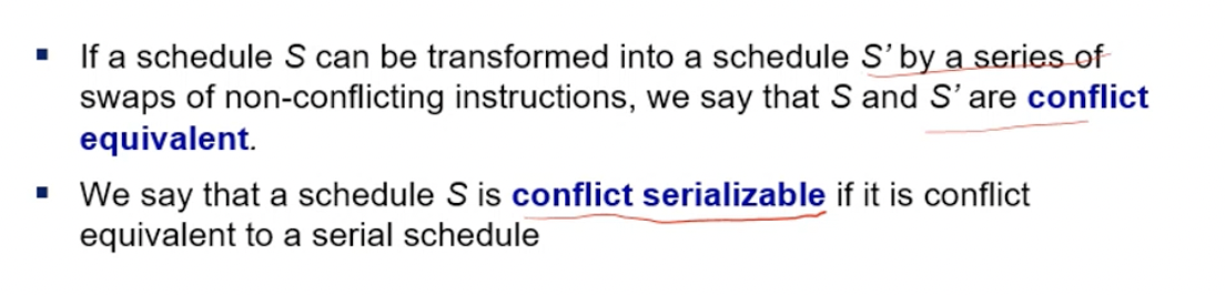
We are skipping view equivalence. There are other notions of serialisability (considering a group of operations).
Testing for Conflict Serialisability
A precedence graph is a directed graph where vertices are transaction IDs and edges represent conflicting instructions with arrows showing the temporal order. Then, we can perform topological sorting to check for serialisability. A schedule is serialisability iff its precedence graph is acyclic.
Lecture 35
04-04-22
We shall discuss a series of concepts in isolation now.
Recoverable Schedules
If a transaction \(T_i\) reads a data item previously written by a transaction \(T_j\), then the commit operation of \(T_j\) appears before the commit operation of \(T_i\). These schedules are recoverable.
Cascading rollbacks
A single transaction failure leads to a series of transaction rollbacks. That is, uncommitted transactions must be rolled back.
Cascadeless Schedules
Cascading rollbacks cannot occur in these schedules. For each pair of transactions \(T_i\) and \(T_j\) such that \(T_j\) reads a data item previously written by \(T_i\), the commit operation \(T_i\) appears before the read operation of \(T_j\). That is, they allow reading of committed values only and disallow dirty reads. Every cascadeless schedule is recoverable.
Weak levels of Isolation
Some applications can tolerate schedules that are not serialisable. For example, in statistics we only want approximations. Ideally, we’d like serialisable, recoverable and preferably cascadable.
There are levels of isolation defined in SQL-92 like - read committed, read uncommitted, repeatable read, and serialisable. Most often, databases run in read committed mode.
Concurrency Control Mechanisms
We have a ton of theory for implementing whatever we have discussed. There are locking schemes, timestamp schemes, optimistic/lazy schemes and multi-versions (similar to master-slave mechanism in parallel cores of architecture).
Transactions in SQL
We have predicate operations in SQL. A tuple might fail a predicate before a transaction, but passes it after the transaction has completed. Some databases lock the matched tuples for consistency, but that does not always work. That is, we need “predicate locking”, not just key-based locks that locks all possible matching tuples. Phantom reads refer to not matching tuples that are just added.
In SQL, a transaction begins implicitly. commit work commits current transaction and begins a new one. rollback work causes current transaction to abort. Isolation levels can be set at database level or at the start of a transaction.
~Chapter 18: Concurrency Control
Lock based protocols
A lock is a mechanism to control concurrent access to a data item. Items can be locked in two modes
- exclusive (X) mode - Data item can be both read as well as written.
lock-X - shared (S) mode - Data item can only be read.
lock-S
These requests are made implicitly using a concurrency control manager. Not that X lock can’t be obtained when a S lock is held on an item.
A locking protocol is a set of rules followed by all transactions while requesting and releasing locks. They enforce serialisability by restricting the set of possible schedules. To handle deadlocks, we need to roll back some transactions. Starvation is also possible if concurrency control manager is badly designed. This occurs because X-locks can’t be granted when S-lock is being used.
Two-Phase Locking Protocol
This protocol ensures conflict-serialisable schedules. We have two phases
- Phase 1: Growing phase. A transaction can obtain locks but not release them
- Phase 2: Shrinking phase. It’s the opposite of the above.
The transactions can be serialised in the order of their lock points (the point where a transaction has acquired its final lock). However, this protocol does not ensure protection from deadlocks. It also does not ensure recoverability. There are extensions that ensure recoverability from cascading roll-back.
- Strict two-phase locking - A transaction must hold all its exclusive locks till it commits/aborts.
- Rigorous two-phase locking - A transaction must hold all locks till commit/abort.
We mostly use the second protocol.
Two-phase locking is not necessary condition for serialisability. That is, there are conflict serialisable schedules that cannot be obtained if the two-phase locking protocol is used.
Given a locking protocol, a schedule \(S\) is legal under a locking protocol if it can be generated by a set of transactions that follow the protocol. A protocol ensures serialisability if all legal schedules under that protocol are serialisable.
In the two-phase locking protocol. we can upgrade (S to X) in the growing phase and downgrade (X to S) in the shrinking phase.
Lecture 36
05-04-22
Implementation of Locking
A lock manager can be implemented as a separate process. The lock manager maintains an in-memory data-structure called a lock table to record granted locks and pending requests. A lock table is implemented as a hash table with queues.
Graph-Based Protocols
They impose a partial ordering \(\to\) on the set \(D = \{d_1, \dots, d_n\}\) of all the data items. If \(d_i \to d_j\), then any transaction accessing both \(f_i\) and \(f_j\) must access \(d_i\) before accessing \(d_j\).
A tree protocol ensures conflict serialisability as well as freedom from deadlock. However, it does not guarantee recoverability and it has other issues.
Deadlocks
There are other deadlock prevention strategies like
- wait-die - non-preemptive. Older transaction may wait for younger one to release the data item, and the younger transaction never wait for older ones. They are rolled back instead.
- wound-wait - preemptive. Older transaction wounds (forces rollback) of a younger transaction instead of waiting for it.
In both the schemes, a rolled back transaction restarts with its original timestamp.
- Time-out based schemes
Deadlock Recovery
There are two ways for rollback
- Total rollback
- Partial rollback - Roll back victim transaction only as far as necessary to release locks that another transaction in cycle is waiting for.
A solution for starvation is that the oldest transaction in the deadlock set is never chosen as victim of rollback.
Multiple Granularity
A lock table might be flooded with entries when a transaction requires coarser granularity. The levels of granularity we use are database, area, file and record. What if we only use coarse granularities? The problem is that it’s not effective in terms of concurrency.
We use intention locks to take care of hierarchy of granularities.
Intention Lock Modes
In addition to S and X, we have
- Intention-shared IS - Indicates explicit locking at a lower level of the tree but only with shared locks.
- Intention-exclusive IX - Indicates explicit locking at a lower level with exclusive or shared locks.
- Shared and intention exclusive SIX - The subtree rooted by that node is locked explicitly in shared mode and explicit locking is being done at a lower level with exclusive-mode locks.
Intention locks allow a higher level node to be locked in S or X mode without having to check all descendent nodes. That is, to get a lock at the bottom level, we need to start taking intention locks from the root. Also, we have the following compatibility matrix.
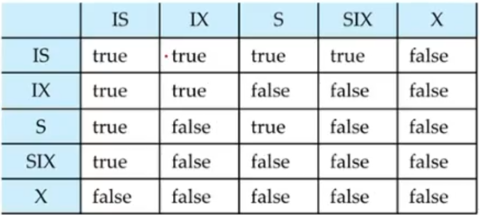
The query engine decides all the locks based on the input queries. It follows adaptive lock granularity when it can’t decide. There is also a notion of lock granularity escalation in adaptive locking where the query engine shifts to a coarser granularity in case there are too many locks at a particular level.
Now, we discuss locking in the case of predicate reads. Consider an insert. You can lock the entire relation to ensure consistency, but when someone inserts a new record there won’t be any lock on it. So, we use the following rules.
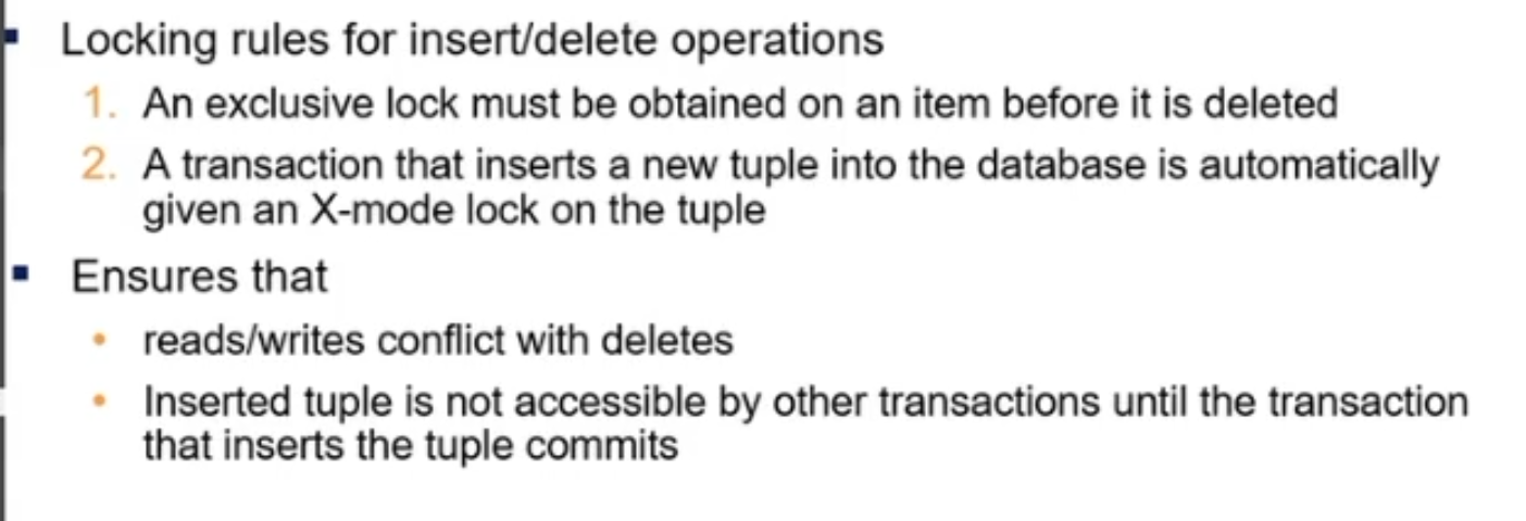
Note that one also locks the metadata in two-phase locking scheme that helps it ensure serialisability.
Phantom Phenomenon
A transaction \(T_1\) performs a predicate read, and a transaction \(T_2\) inserts a matching tuple while \(T_1\) is active but after predicate read. As a result, some of these schedules are not serialisable.
Handling Phantoms
If the conflict is at the data level, locking the metadata will prevent insertion and deletion in the relation. However, this provides very low concurrency for insertions and deletions.
Index Locking to prevent Phantoms
Every relation must have at least one index. A transaction \(T_i\) that performs a lookup must lock all the index leaf nodes that it accesses in \(S\)-mode. That is, it locks a range. A transaction \(T_j\) that inserts, updates or deletes a tuple \(t_i\) in a relation \(r\) must update all indices to \(r\). It can’t acquire X-lock in the locked range of \(T_i\). So phantom reads won’t occur when the rules of two-phase locking protocol must be observed. The key idea here is that, tuples in the matching range will be sequential do to the index.
Next-Key Locking to prevent Phantoms
This method provides higher concurrency. It locks all values that satisfy index lookup, and also lock the next key value in the index.
Note that the above locks are done in the \(B^+\) trees.
Lecture 37
07-04-22
Timestamp Ordering Protocol
The timestamp-ordering protocol guarantees serialisability since all the arcs in the precedence graph are of the form having nodes with edges from smaller timestamp to larger timestamp. This protocol ensures freedom from deadlock as no transaction ever waits. However, the schedule may not be cascade free and may not even be recoverable.
To make it recoverable, we have the following solutions
- All the writes are done at the end of the timestamp. A transaction that aborts is restarted with a new timestamp.
- Limited form of locking - wait for data to be committed before reading it
- Use commit dependencies to ensure responsibility.
Thomas’ Write Rule
Modified version of the TSO in which obsolete write operations may be ignored under certain circumstances. When a transaction items to write to a data item Q which will be rewritten by another transaction, then the original write is considered as obsolete. \(TS(T) < W_\text{timestamp}(Q)\). So, rather than rolling back the original transaction as the TSO does, we ignore the write operation in the original transaction. In this way, Thomas’ Write Rules allows greater potential concurrency. It allows some view serialisable schedules that are not conflict-serialisable.
The rule comes into the picture in case of blind writes - A write is done without a preceding read.
Validation Based Protocol
It uses timestamps, but they are not pre-decided. The validation is performed at commit time to detect any out-of-serialisation order reads/writes. It is also known as optimistic concurrency control since transaction executes fully in the hope that all will go well during validation. This is done in three phases
- Read and execution phase. Writes are done to temporary variables.
- Validation phase
- Write phase
Each transaction has 3 timestamps corresponding to start of execution, validation phase, and write phase. The validation time stamps are used in the protocol. In validation, we check that for all \(T_i, T_j\) such that \(TS(T_i) < TS(T_j)\), one of the following must hold
- \[finishTS(T_i) < startTS(T_j)\]
- \(startTS(T_j) < finishTS(T_i) < validationTS(T_j)\) and the set of data items written by \(T_i\) does not intersect with the set of data items read by \(T_j\).
This is when the validation succeeds.
Multiversion Concurrency Control
Multiversion schemes keep old versions of data item to increase concurrency. There are variants such as
- Multiversion Timestamp Ordering
- Multiversion Two-Phase Locking
- Snapshot isolation
The key ideas are that
- Each successful write results in the creation of a new version that labeled using timestamps.
- When a read operation is issued, we select the appropriate timestamp based on the timestamp of transaction issuing read and return the value of the selected version.
Multiversion Timestamp ordering
Each data item \(Q\) has a sequence of versions \(< Q_1, \dots, Q_n>\) each of which have
- Content
- Write timestamp
- Read timestamp
If \(T\) issues a read or write, let \(Q_k\) be the version with the highest write timestamp that has a value less than the timestamp of \(T\). Then for a read, we return the value from \(Q_k\), and for a write we overwrite if both the timestamps are equal. We roll back \(T\) if \(TS(T) < R\_timestamp\). Otherwise, we simply create a new entry.
Like the basic TSP, recoverability is not ensured.
Multiversion Two-Phase Locking
Differentiates between read-only transactions and update transactions. Update transactions follow rigorous two-phase locking. Read of a data item returns the latest version of the item. The first write of \(Q\) by \(T\) results in creation of a new version \(Q_i\) and the timestamp is updated after the completion of the transaction. After the transaction \(T\) completes, \(TS(T_i) = \texttt{ts-counter} + 1\) and \(W\_timestamp(Q) = TS(T_i)\) for all versions of \(Q\) that it creates. Then, the ts-counter is incremented. All of this must be done atomically.
In read only transactions, ts-counter is assigned to the timestamp. As a result, only serialisable schedules are produced.
The issues with multiversion schemes are they increase storage overhead and there are issues with keys constraint checking and indexing with multiple versions.
Snapshot Isolation
A transaction \(T\) executing with snapshot isolation
- Takes snapshot of the committed data at start
- Always reads/modified data in its own snapshot
- Updates of concurrent transactions are not visible to \(T\)
- Writes of \(T\) are complete when it commits
So, first committer wins rule is being used. Serialisable snapshot isolation (SSI) is an extension that ensures serialisability. However, there are some anomalies in this.
Lecture 38
11-04-22
~Chapter 19:
A transaction failure can occur as a result of
- logical errors - internal error condition in the transaction. These can be somewhat prevented by
assertstatements. - system error - database must terminate the transaction due to errors like deadlock.
System crash - Occurs due to a power failure, hardware or software failure. A failstop assumption refers to the assumptions that non-volatile storage contents are not corrupted by a system crash. A disk failure destroys disk storage.
Logging helps in recovery. To recover from failure, we first find inconsistent blocks by
- We compare two copies of every disk block which is expensive, or
- Use logs sort of mechanism
and then overwrite the inconsistent blocks. We also need to ensure atomicity despite failures.
Log-Based Recovery
A log is a sequence of log records that keep information of update activities on the database. When transaction \(T\) starts, it registers itself by writing \((T start)\) log record. Before \(T\) executes \(write(X)\), it writes a log record \((T, X, V_1, V_2)\). Upon finishing the last statement, the log record \((T commit)\) is written. There are two approaches using log
- Immediate database modification - write to buffer which will write to disk when before the transaction commits. Log record is written before database item is written.
- Deferred database modification - writes are done only after commit. Not used frequently.
A transaction is said to have committed when its commit log record is output to stable storage. Also, the log records are interleaved for concurrent transactions.
Concurrency Control and Recovery
We assume that if a transaction \(T\) has modified an item, no other transaction can modify the same item until \(T\) has committed or aborted. This is equivalent to strict two phase locking.
- \(undo(T_i)\) restores the value of all data items updated by \(T_i\) to their old values, going backwards from the last log record for \(T_i\). For each restoration, we add a log record of \((T_i, X, V)\). When undo of a transaction is complete, a log record \((T_i abort)\) is written out.
- \(redo(T_i)\) sets the value of all data items updated by \(T_i\) to the new values, going forward from the first log record of \(T_i\). The log is unchanged here.
Recovering from Failure
When recovering from failure,
- Transaction \(T_i\) needs to be undone if the log contains the record \((T_i start)\) but does not contain \((T_i commit)\) or \((T_i abort)\)
- It needs to be redone if it contains \((T_i start)\) and \((T_i commit)\) or \((T_i abort)\).
Note that the second step is wasteful in some cases. We recovered before, and we are doing it again. This is known as repeating history.
Checkpoints
Processing the entire log can be slow. We streamline recovery procedures by periodically performing checkpointing.
- Output all log records currently residing in the main memory onto stable storage
- Output all modified buffer blocks to the disk
- Write a log record \((checkpoint L)\) onto stable storage where \(L\) is a list of all transactions active at the time of checkpoint
- All updates are stopped while doing checkpointing.
The log records before a checkpoint are not needed!
Lecture 39
12-04-22
## Recovery Algorithm
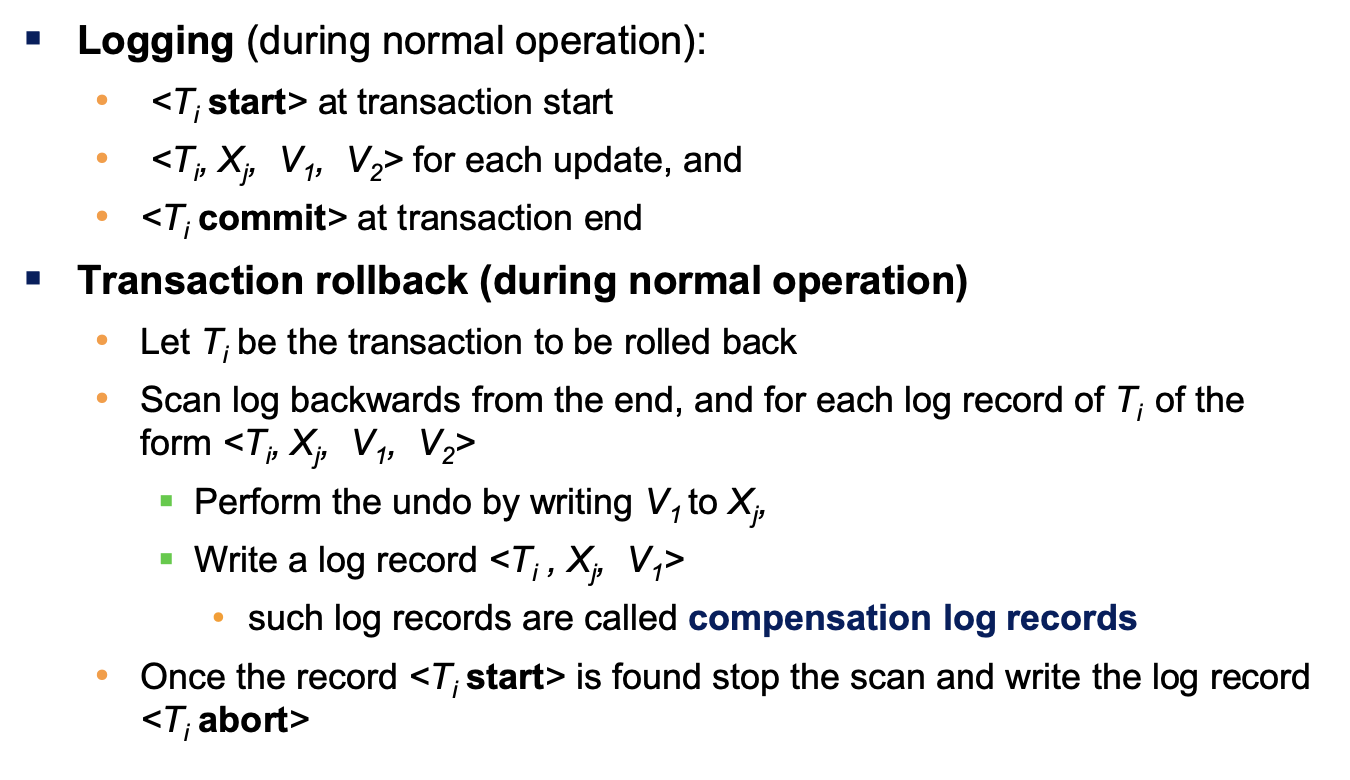
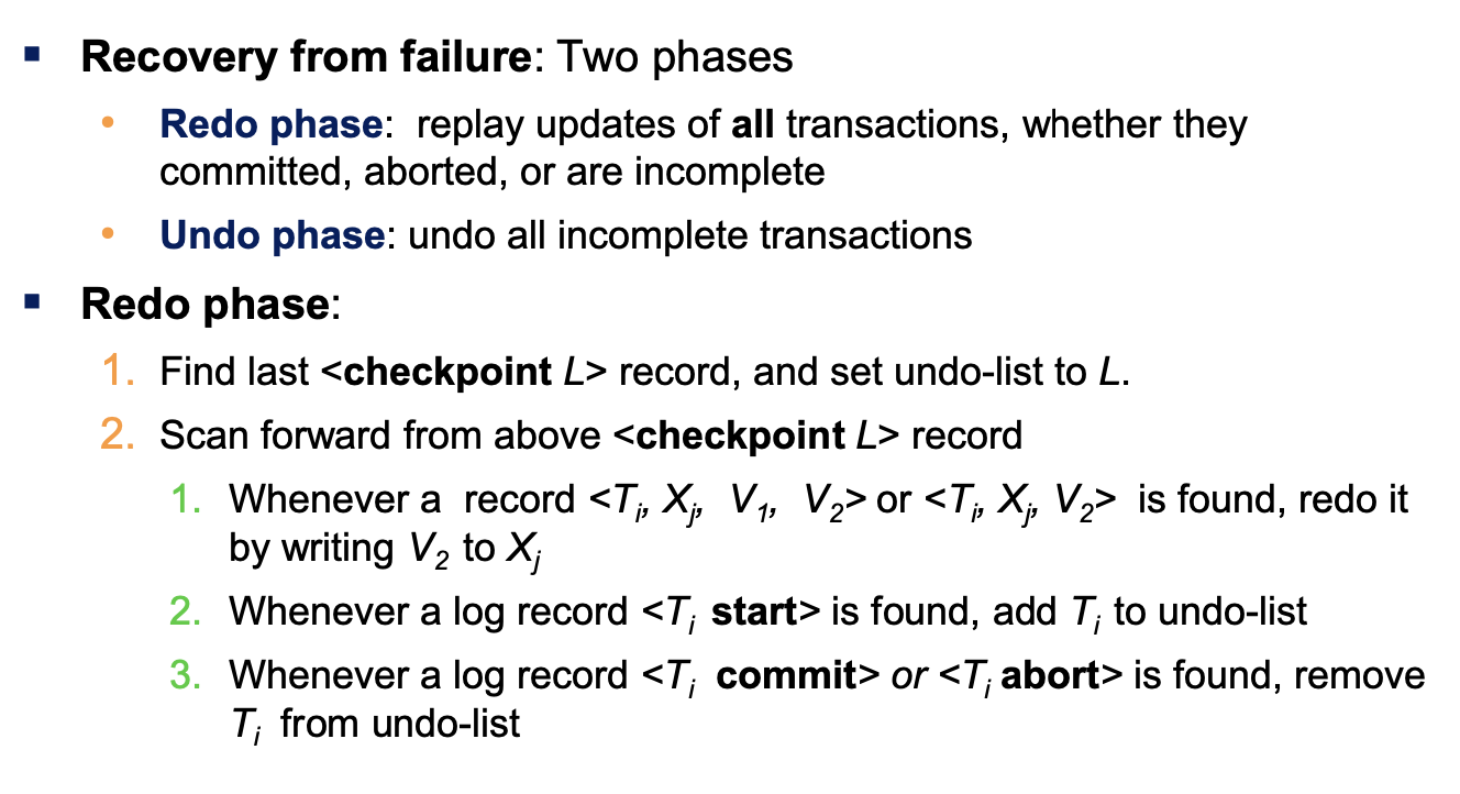
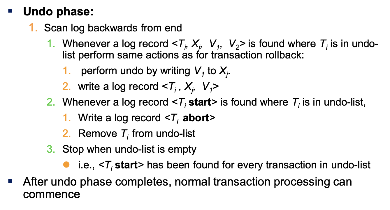
Log Record Buffering
Log records are buffered in main memory, instead of being output directly to stable storage. When the buffer is full, a log force operation is performed.
As we had said, before a block of data in the main memory is output to the database, all log records pertaining to data in that block must have been output to stable storage. This rule is called as write-ahead logging or WAL rule. Strictly speaking, this is only required for undo transactions.
Database Buffering
The recovery algorithm supports the no-force policy - updated blocks need not be written to disk when transaction commits. However, force policy is a more expensive commit. The recovery algorithm also supports the steal policy - blocks containing updates of uncommitted transactions can be written to disk, even before the transaction commits.
No updates should be in progress on a block when it is output to disk. It can be ensured by acquiring exclusive locks on the block before writing a data item. Locks can be released once the write is completed. Such locks held for short durations are called latches.
In summary, we acquire latch, do log flush, write block to disk and finally release the latch.
The dual paging problem refers to the extra I/O that is done when fetching a page from swap to buffer and then moving it to the disk. This can be prevented by letting the OS pass the control to the database when it needs to evict a page from the buffer. The database outputs the page to the database instead of the swap space, and release the page from the buffer.
Fuzzy Checkpointing
to avoid long interruption of normal processing during checkpointing, we allow updates to happen during checkpointing. We permit transactions to proceed with their actions once we note the list \(M\) of modified buffer blocks. We store a pointer to the checkpoint record in a fixed position last_checkpoint on disk once the all modified buffer blocks in \(M\) are output to disk. During recovery, we use this last checkpoint.
Failure with Loss of Nonvolatile Storage
Technique similar to checkpointing used to deal with the loss of non-volatile storage. That is, we periodically dump the entire content of the database to stable storage. No transaction may be active during the dump procedure. We perform the following -
- output all log records from main memory to storage
- output all buffer blocks onto the disk
- copy the contents of the database to stable storage
- output a record \((dump)\) to lon on stable storage.
There are versions of fuzzy dump and online dump.
Remote Backup Systems
We need to detect failure at the backup site using heartbeat messages and perform transfer of control to take control at the backup site. The log records are copied at the backup before, and recovery can be initiated. Once the primary site goes back up, we give back the control.
The time to recover is very important to reduce delay in takeover. Therefore, the backup sire periodically processed the redo log records, performs a checkpoint, and can then delete earlier parts of the log.
A hot-spare configuration permits very fast takeover - backup continually processes redo logs as they arrive and when the failure is detected, the backup rolls back incomplete transactions and is ready to process new transactions. An alternative to remote system backup is to use distributed systems.
We have the following levels of durability
- One safe - Commit as soon as transaction’s commit log record is written at primary.
- Two-very safe - Commit when transaction’s commit log record is written at primary and backup.
- Two-safe - Proceed as in two-very-safe is both primary and backup are active.
We also need to reduce latency for communication. We add a near site backup close to the primary site. Log records are replicated both at near site and remote backup site. If primary fails, remote backup site gets latest log records, which it may have missed, from near site.
END OF COURSE
Enjoy Reading This Article?
Here are some more articles you might like to read next: