IPL Notes
Lecture 1
05-01-22
Binding
Binding refers to finding certain attributes of certain objects. For example, when we consider the example of developing a program, we have the following steps.
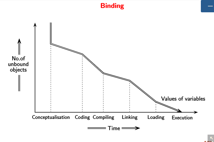
At each step, the number of unbound objects decrease along with time.
Implementation Mechanisms
The important point to note is that the “execution” is done after “translation” in the case of compilers (Analysis + Synthesis). However, interpreters (Analysis + Execution) themselves are programs which take the source code as input and translate/execute the user-program.
Compilers/Translators lower the level of the program specification, whereas the interpreters do the opposite. That is why interpreters are able to directly execute the source code.
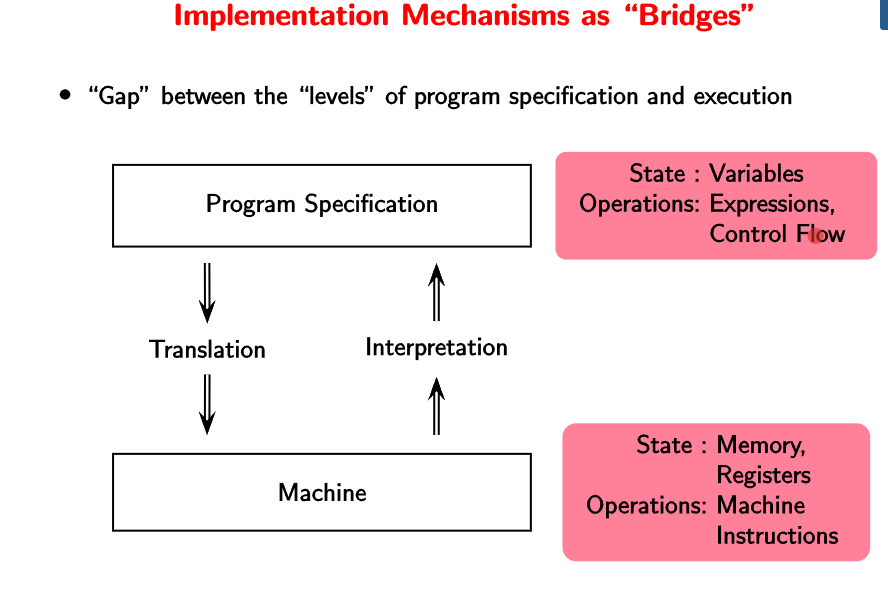
Why is the arrow in the reverse direction? Think of python. The python program itself is a low-level code which is able to execute a high-level user code.
| High Level | Low Level |
|---|---|
| C statements | Assembly statement |
Note. A practical interpreter does partial translation/compilation but not completely as it is redundant.
Compilers performs bindings before runtime, and an interpreter performs bindings at runtime.
Why interpreters if compilers are fast? Compilers are used for programs which need to be executed multiple times with speed. However, we must also consider the time needed to compiler the codes in case of compilers. Considering this, the turnaround time in both cases is almost the same. The user needs to think whether they want to reduce the execution time or reduce the turnaround time.
| Language | Mode of execution |
|---|---|
| C++ | Compiler |
| Java/ C# | Compiler + Interpreter |
| Python | Interpreter |
Java programs run on a virtual machine - JIT (just in time) compilation. the virtual machine invokes a native compiler for instances of code which are repeated often inside the code. This speeds up the execution in case of Java.
Compilers like GCC can be used for multiple machines and languages. 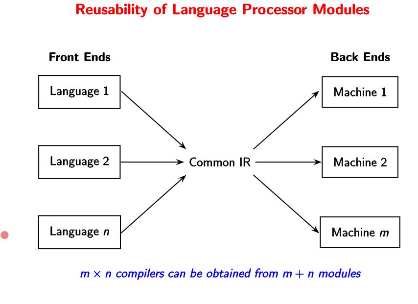
Simple compiler
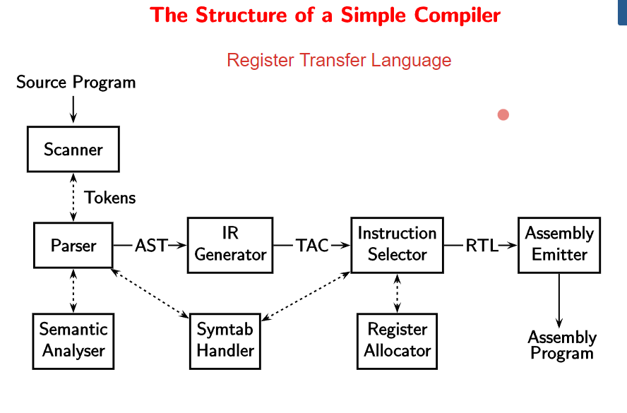
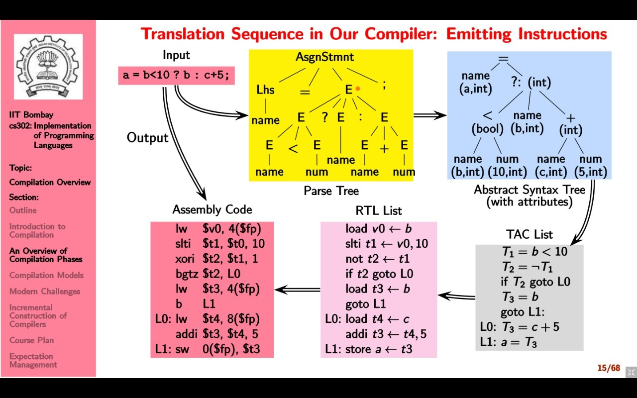
The first step in the translation sequence of the compiler is scanning and parsing. A parse-tree is built from the grammar rules, terminals, and non-terminals. Scanning involves finding special characters to create the parse tree, whereas parsing is essentially creating the parse tree itself.
The next step involves semantic analysis. The semantic analyzer performs type checking to check the validity of the expressions. Therefore, we create an abstract syntax tree (AST) is created from the parse tree.
Only for type-checking? Yes, that is the primary purpose, but it has other uses too. Sometimes, type checking is done on the fly while generating the parse tree itself. The advantage for generating the AST is that we can write a generic code (interpreter) to parse the abstract trees (since it involves only tokens).
Then, we generate a TAC list (three address code) in the IR generation step. This step helps in separating data and control flow, and hence simplifies optimization. The control flow is linearized by flattening nested control constructs.
In the Instruction Selection step, we generate the RTL list which is like pseudo-assembly code with all the assembly instruction names. We try to generate as few instructions as possible using temporaries and local registers.
What is the purpose of this step? We like to divide the problem into many steps to leave room for optimization.
In the final step of Emitting Instructions, we generate the assembly code by converting the names of assembly instructions to the actual code.
The whole process is summarized by the following image.
Observations
A compiler bridges the gap between source program and target program. Compilation involves gradual lowering of levels of the IR of an input program. The design of the IRs is the most critical part of a compiler design. Practical compilers are desired to be retargetable.
Lecture 2
07-01-22
Write about retargetable compilers. A retargetable compiler does not require manual changes, the backend is generated according to the specifications.
Why are compilers relevant today?
In the present age, very few people write compilers. However, translation and interpretation are fundamental to CS at a conceptual level. It helps us understand stepwise refinement - building layers of abstractions and bridging the gaps between successive layers without performance penalties. Also, knowing compilers internals makes a person a much better programmer.
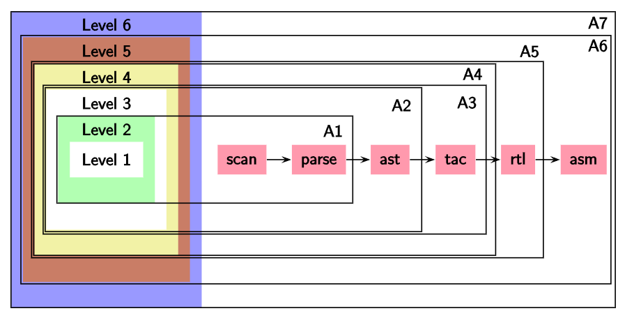
Modularity of Compilation
A compiler works in phases to map source features to target features. We divide each feature into multiple levels for convenience. This will be clear through the assignments (language increments).
Course Plan
We shall cover scanning, parsing, static semantics, runtime support, and code generations in the theory course. In the lab course, we shall do incremental construction of SCLP.
Lecture 3
12-01-22
Compilation Models
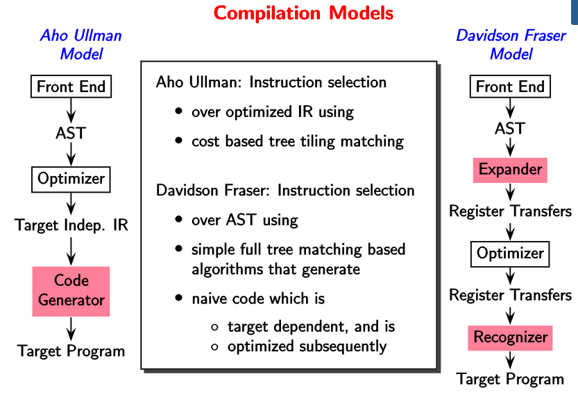
Registers are introduced earlier in the Davidson Fraser model. Therefore, it becomes machine dependent. The target independent IR in gcc is called ‘gimple’.
Typical Front ends
How does a front end work? Usually, the parser calls the scanner that reads the source program to extract tokens. These tokens are then used by the parser to create the parse tree. We can say that the scanner is a subordinate routine of the parser. On the other side, the parser sends the parse tree to the semantic analyzer which generates the AST. Finally, we get the AST/ Linear IR along with a symbol table.
Typical Back ends in Aho Ullman Model
The backend receives the machine independent IR from the front end. It then proceeds to optimize the instructions via compile time evaluations and elimination of redundant computations. There are techniques such as constant propagation and dead-code elimination that are used.
After optimization, the code generator converts the machine independent IR to machine dependent IR. The essential operations done by the code generator are instruction selection, local register allocation, and the choice of order of evaluation.
Finally, we have the machine dependent optimizer which outputs assembly code. It involves register allocators, instruction schedulers and peephole optimizer.
GNU Tool Chain for C
We know that the gcc compiler take source program as input and produces a target program. Internally, this is done via a compiler called ‘cc1’ (C compiler 1) which generates the assembly program. This assembly code is taken by the assembly component of the compiler to generate an object file. Finally, the loader takes this object file along with glibc/newlib to generate the target program. The assembly program and loader together are known as binutils.
LLVM Tool Chain for C
The LLVM tool chain looks similar to the GNU tool chain. We have clang -cc1, clang -E, llvm-as (assembly program) and lld(loader). The re-targetability mechanism is done via table generation code.
Modern Challenges
Currently, most of the implementation of compilers has been more or less done. What is left? Some applications and architectures demand special programming languages and compilers that are non-standard. Also, there are some design issues with compilers. It is the IR that breaks or makes a compiler. Including these there are many places of optimization such as
- Scaling analysis to large programs without losing precision
- Increasing the precision of analysis
- Combining static and dynamic analysis.
Full Employment Guarantee Theorem for Compiler Writers.
- Software view is stable, hardware view is disruptive.
- Correctness of optimizations
- Interference with security
- Compiler verification and Translation Validation
- Machine Learning?
- \[\dots\]
~ Lexical Analysis
Scanners
To discover the structure of the program, we first get a sequence of lexemes or tokens using the smallest meaningful units. Once this is done, we remove spaces and other whitespace characters in the lexical analysis or scanning step.
In the second step, we group the lexemes to form larger structures (parse tree). This is called as syntax analysis or parsing. There are tools like Antlr that combine scanning with parsing.
Lexemes, Tokens, and Patterns
Definition. Lexical Analysis is the operation of dividing the input program into a sequence of lexemes (tokens). Lexemes are the smallest logical units (words) of a program. Whereas, tokens are sets of similar lexemes, i.e. lexemes which have a common syntactic description.
How are tokens and lexemes decided? What is the basis for grouping lexemes into tokens? Generally, lexemes which play similar roles during syntax analysis are grouped into a common token. Each keyword plays a different role and are therefore a token by themselves. Each punctuation symbol and each delimiter is a token by itself All comments are uniformly ignored and hence are grouped under the same token. All identifiers (names) are grouped in a common token.
Lexemes such as comments and white spaces are not passed to the later stages of a compiler. These have to be detected and ignored. Apart from the token itself, the lexical analyzer also passes other information regarding the token. These items of information are called token attributes.
In conclusion, the lexical analyzer
- Detects the next lexeme
- Categorizes it into the right oken
- Passes to the syntax analyzer. The token name for further syntax analysis and the lexeme itself.
Lecture 4
19-01-22
Creating a lexical analyzer
- Hand code - possible more efficient but seldom used nowadays.
- Use a generator - Generates from formal description. Less prone to errors.
A formal description of the tokens of the source language will consist of
- A regular expression describing each token, and
- A code fragment called an action routine describing the action to be performed, on identifying each token.
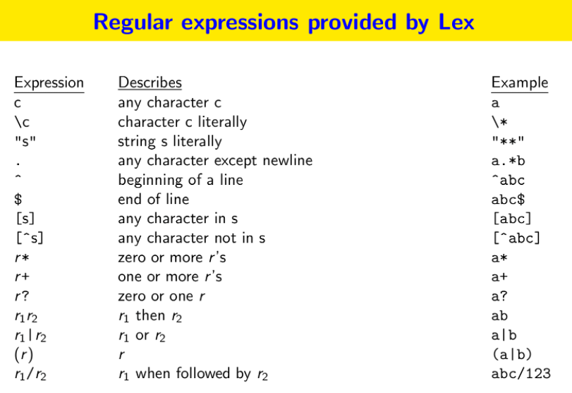
Some regex notation -
- Alternation is represented using
| - Grouping is done via parentheses
-
+is positive closure and*is Kleene closure
The generator, such as Lex, puts together
- A DFA constructed from the token specification
- A code fragment called a driver routine which can traverse any DFA
- Action routines associated with each regular expression.
Usually, the lexeme with the longest matching pattern is taken into consideration.
Regular Expressions
A regular expression is a set of strings (a language) that belongs to set formed the following rules
- \(\epsilon\) and single letters are regular expressions.
- If \(r, s\) are regular expressions, then \(r\vert s\) is a regular expression. That is, \(L(r\vert s) = L(r) \cup L(s)\)
- If \(r,s\) are regular expressions, then \(rs\) is a regular expression. That is, \(L(rs) =\) concatenation of strings in \(L(r)\) and \(L(s)\).
- If \(r\) is a regular expression then \(r^*\) is a regular expression. That is, \(L(r^*)\) is the concatenation of zero or more strings from \(L(r)\). Similarly, for \(r^+\)
- If \(r\) is a regular expression, then so is \((r)\).
The syntax of regular expressions according to Lex is given as
The return statements in the action routines are useful when a lexical analyzer is used in conjunction with a parser. Some conventions followed by lexical analyzers are
- Starting from an input position, detect the longest lexeme that could match a pattern.
- If a lexeme matches more than one pattern, declare the lexeme to have matched the earliest pattern.
Lexical errors
There are primarily three kinds of errors.
- Lexemes whose length exceeds the bound specified by the language. Most languages have a bound on the precision of numeric constants. This problem is due to the finite size of parse tables.
- Illegal characters in the program.
- Unterminated strings or comments.
We could issue an appropriate error message to handle errors.
Lecture 5
21-01-22
Tokenizing the input using DFAs
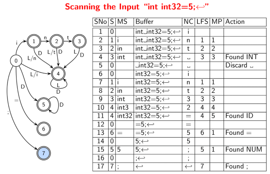
The format to show a trace of scanning is given by
| Step No | State | Matched String | Buffer | NextChar | LastFinalState | MarkedPos | Action | | ——- | —– | ————– | —— | ———- | —————- | ———– | —— |
Here, MatchedString is the prefix of the buffer matched to identify a lexeme. NextChar is the next character in the input; it will be shifted to the buffer if there is a valid transition in the DFA. MarkedPos is the position of the character (in the buffer) just after the last seen lexeme. The important point to note is that when there is no transition on Nextchar,
- if
MarkedPosis -1, no final state was seen, the first character in the buffer is discarded, and the second character becomesNextChar. - otherwise, the lexeme up to
MarkedPos(excluding it) is returned, the character atMarkedPosbecomesNextChar.
In either case, the LastFinalState is set to -1 and the state is set to 0. See the following example for clarity.
This sort of parsing has quadratic behavior in the worst case. Consider the following two questions.
- Is \(S\) always equal to
LastFinalState? - Is
MPalways equal to the length of the last lexeme?
The answer to both questions is “No”. Think.
~ Introduction to Parsing using Lex/Flex and Yacc/Bison
Lex is a program that takes regular expressions as input and generates a scanner code. A Lex script can be decoded as follows. It has three parts separated by “%%”.
- The first part consists of declarations. These are copied to
lex.yy.cand are contained in the pair “%{” and “%}”. Declarations outside of this pair are directives to lex or macros to be used in regular expressions. - The second part consists of rules and actions. These are basically a sequence of “Regex SPACE Action” lines.
- Finally, the third part consists of auxiliary code.
Yacc is a program that takes tokens from the scanner and parses them. A yacc script is very similar to that of lex. It has three parts which are separated by “%%”.
- The first part has declarations that are to be copied to
y.tab.ccontained in the pair “%{” and “%}”. Declarations outside of this pair are directives to yacc or specifications of tokens, types of values of grammar symbol, precedence, associativity etc. - The second part has rules and actions. That is, a sequence of grammar productions and actions.
- The last part has the auxiliary code.
The yacc and lex scripts are combined together using gcc. The typical workflow is
yacc -dv <file-name>.y
gcc -c y.tab.c
lex <file-name>.l
gcc -c lex.yy.c
gcc -o <obj-file-name> lex.yy.o y.tab.o -ly -ll
Lecture 6
29-01-22
A parser identifies the relationship between tokens.
Constructing DFAs for Multiple Patterns
- Firstly, join multiple DFAs/NFAs using \(\epsilon\) transitions.
- This creates an NFA. This NFA can be converted to a DFA by subset construction. Each state in the resulting DFA is a set of “similar” states of the NFA. The start state of the DFA is a union of all original start states (of multiple patterns). The subsequent states are identified by finding out the sets of states of the NFA for each possible input symbol.
Constructing NFA for a Regular Expression
Consider a regular expression \(R\).
- If \(R\) is a letter in the alphabet \(\Sigma\), create a two state NFA that accepts the letter.
- If \(R\) is \(R_1.R_2\), create an NFA by joining the two NFAs \(N_1\) and \(N_2\) by adding an epsilon transition from every final state of \(N_1\) to the start state of \(N_2\).
- If \(R\) is \(R_1\vert R_2\), create an NFA by creating a new start state \(s_0\) and a new final state \(s_f\). Add an epsilon transition from \(s_0\) to the start state of \(R_1\) and similarly for \(R_2\). Also, add an epsilon transition from every final state of \(N_1\) to \(s_f\) and similarly for \(N_2\).
- If \(R\) is \(R_1^*\), create an NFA by adding an epsilon transition from every final state of \(R_1\) to the start state of \(R_1\).
- In the 2nd rule, all the final states in \(N_1\) must be made into normal states?
- In the 4th rule, \(R\) must accept \(S = \epsilon\) too.
- Where is the rule for \(R = (R_1)\).
Recall the following rules
-
First matching rule preferred. For example, if we write the rule $$L(L D)^*\(- ID before\)int\(- INT, then the lexeme\)int$$ will be taken as ID token and not INT token. - Longest match preferred. For example, consider identifiers and int and the lexeme \(integer\). Then the lexeme will be treated as a single identifier token, and not an INT followed by ID.
These rules are implicitly a part of DFAs in a way. The construction ensures the longest match is preferred. The accepted pattern is chosen from the possible patterns based on the first matching rule. To ensure our grammar works as intended, special patterns must be written before general patterns.
Representing DFAs using Four Arrays
A parsing table is also represented in a similar way. This is a general efficient representation for sparse data. The representation is explained through an example. Consider the following DFA
| a | b | c | |
|---|---|---|---|
| 0 | 1 | 0 | 3 |
| 1 | 1 | 2 | 3 |
| 2 | 1 | 3 | 3 |
| 3 | 1 | 0 | 3 |
with \(2\) being the final state. We use the following character codes
| Char | Code |
|---|---|
| a | 0 |
| b | 1 |
| c | 2 |
Notice that states 0 and 3 have identical transitions. States 1 and 2 differ only on the ‘b’ transition. We shall use these similarities to exploit compact representation. The four arrays we consider are default, base, next and check. We follow the given steps.
- We choose to fill the entries for state 0 first.
- The ‘check’ array contains 0 to confirm that the corresponding entries in the ‘next’ array are for state 0. ‘Base’ is the location from which the transitions of state are stored in the ‘next’ array.
- For state 1, we reuse the transition on a and c from state 0 but we need to enter transition on b explicitly. We do this using the next free entry in the next array and back calculating the base of state 1.
- State 2 is filled in the same way.
- State 3 is identical to state 0. We keep its base same as that of state 0.
The transition function in pseudocode is given by
int nextState(state, char)
{
	if (Check[Base[state] + char] == state)
        return Next[Base[state] + char];
    else
    	return nextState(Default[state], char);
}
How do we prevent clashes in the next array?
We can further compress the tables using equivalence class reduction. In the above code, instead of char, we can have class. So for example, instead of defining transitions separately for 26 characters, we can define a single transition for all the letters. Further optimization can be done via meta-equivalence classes.
Lecture 7
02-02-22
Syntax Analysis
We had seen Lexical analysis so far. Syntax analysis discovers the larger structures in a program.
A syntax analyzer or parser
- Ensures that the input program is well-formed by attempting to group tokens according to certain rules. This is syntax checking.
- Creates a hierarchical structure that arises out of such grouping - parse-tree.
Sometimes, parser itself implements semantic-analysis. This way of compiler organization is known as parser driven front-end. On the other hand, if there is a separate semantic analyzer, then the organization is known as parser driven back-end?. Also, if the the entire compilation is interleaved along with parsing, then it is known as parser driven compilation. However, this organization is ineffective as optimizations are not possible.
Till the early 70s, parsers were written manually. Now, plenty of parser generating tools exist such as
- Yacc/Bison - Bottom-up (LALR) parser generator
- Antlr - Top-down (LL) scanner cum parser generate.
- PCCTS, COCO, JavaCC, …
To check whether a program is well-formed requires the specification to be unambiguous, correct and complete, convenient
A context free grammar meets these requirements. Each rule in the grammar is called as a production. The language defined by the grammar is done via the notion of a derivation. That is, the set of all possible terminal strings that can be derived from the start symbol of a CFG is the language of the CFG.
For example, consider the grammar to define the syntax for variable declaration
declaration -> type idlist;
type -> integer | float | string
idlist -> idlist, id | id
Now, the parser can check if a sentence belongs to the grammar to check the correctness of the syntax. However, sometimes our algorithms to check whether a word is present in a grammar don’t work. When the derivations are unambiguous, most of the algorithms work in all cases.
Human language is context-sensitive not context-free. For example, “Kite flies boy” and “boy files kite” are both syntactically correct. Such problems also arise in case of programming languages, but these are easier to deal with. We shall see this issue in Semantic Analysis.
Equivalence of grammars in NP complete.
Why “Context Free”?
The only kind of productions permitted are of the form non-terminal -> sequence of terminals and non-terminals. In a derivation, the replacement is made regardless of the context (symbols surrounding the non-terminal).
Derivation as a relation
A string \(\alpha, \alpha \in (N \cup T)^*\), such that \(S \xrightarrow{*} \alpha\), is called a sentential form of \(G\).
During a derivation, there is a choice of non-terminals to expand at each sentential form. We can arrive at leftmost or rightmost derivations.
Lecture 8
04-02-22
Parse Trees
If a non-terminal \(A\) is replaced using a production \(A \to \alpha\) in a left-sentential form, then \(A\) is also replaced by the same rule in a right-sentential form. The previous statement is only true when there is no ambiguity in derivations. The commonality of the two derivations is expressed as a parse tree.
A parse tree is a pictorial form of depicting a derivation. The root of the tree is labeled with \(S\), and each leaf node is labeled b a token on by \(\epsilon\). An internal node of the tree is labeled by a non-terminal. If an internal node has \(A\) as its label and the children of this node from left to right are labeled with \(X_1, X_2, \dots, X_n\), then there must be a production \(A \to X_1X_2\dots X_n\) where \(X_i\) is a grammar symbol.
Ambiguous Grammars
Consider the grammar
\[E \to E + E \ \vert \ E*E \ \vert \ id\]and the sentence id + id * id. We can have more than one leftmost derivation for this sentence.
The other leftmost derivation is -
\[\begin{align} E &\implies E * E \\ &\implies E + E * E \\ &\implies id + E * E \\ &\implies id + id * id \end{align}\]A grammar is ambiguous, if there is a sentence for which there are
- more than one parse trees, or equivalently
- more than one leftmost/right most derivations.
We can disambiguate the grammar while parsing (easier choice) or the grammar itself.
Grammar rewriting
Ambiguities can be eradicated via
- Precedence
- Associativity
Parsing Strategies
We have top-down and bottom-up parsing techniques. We shall only see bottom-up parsing in this course.
Consider the grammar
D -> var list : type;
tpye -> integer | float;
list -> list, id | id
The bottom-up parse and the sentential forms produced for the string var id, id : integer ; is -
var id, id : integer ;
var list, id : integer ;
var list : integer ;
var list : type ;
D
The sentential forms happen to be a right most derivation reverse order. The basic steps of a bottom-up parser are
- to identify a substring within a rightmost sentential form which matches the rhs of a rules
- when this substring is replaced by the lhs of the matching rule, it must produce the previous rm-sentential form.
Such a substring is called handle.
Handle - A handle of a right sentential form \(\gamma\), is
- a production rule \(A \to \beta\), and
- an occurrence of substring \(\beta\) in \(\gamma\).
Bottom-up parsing is an LR parsing as it amounts to reading the input from left to right, and placing the right most derivation in reverse.
Note. Only terminal symbols can appear to the right of a handle in a right most sentential form.
~ Syntax Analysis
We shall assume that we know how to detect handles in a string, and proceed with parsing algorithms.
Shift Reduce Parsing
Basic actions of the shift-reduce parser are -
- Shift - Moving a single token form the input buffer onto the stack till a handle appears on the stack.
- Reduce - When a handle appears on the stack, it is popped and replaced by the lhs of the corresponding production rule.
- Accept - When the stack contains only the start symbol and input buffer is empty, then we accept declaring a successful parse.
- Error - When neither shift, reduce or accept are possible, we throw an error (syntax).
Lecture 9
09-02-22
Properties of shift-reduce parsers
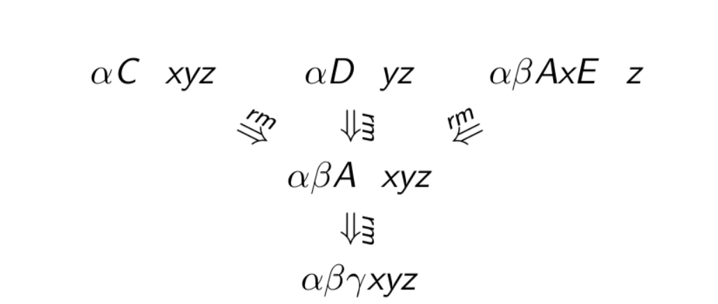
Is the following situation possible?
- \(\alpha \beta \gamma\) is the stack content, and \(A\to \gamma\) is the handle.
- The stack content reduces to \(\alpha \beta A\)
- Now, \(B \to \beta\) in the next handle.
Notice that the handle is buried in the stack. The search for the handle can be expensive. If this is true, then there is a sequence of rightmost derivations
\[S \xrightarrow{*rm} \alpha BAxyz \xrightarrow{rm} \alpha \beta Axyz \xrightarrow{rm} \alpha \beta \gamma xyz\]However, this is not a valid rightmost derivation. Therefore, the above scenario is not possible.
This property does not ensure unique reductions with SR parser. For example, we can have the following.
These problems are collectively grouped as shift-reduce conflicts and reduce-reduce conflicts. Given a parsing table, each (state, char) pair can have two possible valid actions. These conflicts are resolved by conventionally choosing one action over the other.
Simple Right to Left Parsing (SLR(1))
Shift reduce parsing is a precursor to this parsing method. As in, shift reduce parsing does not have a definitive algorithm as such, and it is formalized using SLR parsing.
Shift Reduce Parsing: Formal Algorithms
The first step involves disambiguating the grammar. Shift reduce conflicts are resolved using precedence and associativity. As we have seen, we trace right most derivations in reverse by identifying handles in right sentential forms and pruning them for constructing the previous right sentential form.
How do we identify handles? We need to discover a prefix of right sentential form that ends with a handle.
A viable prefix of a right sentential form that does not extend beyond the handle. It is either a string with no handle, or it is a string that ends with a handle. By suffixing terminal symbols to the viable prefix of the second kind, we can create a right sentential form. The set of viable prefixes forms a regular language (as they are prefixes), thus they can be recognised by a DFA. We keep pushing prefixes on the stack until the handle appears on the top of the stack.
The occurrence of a potential handle does not mean it should be reduced, the next terminal symbol decides whether it is an actual handle. In general, the set of viable prefixes need not be finite and the DFA to recognise them may have cycles.
An item is a grammar production with a dot (\(\bullet\)) in it somewhere in the RHS. The dot separates what has been seen from what may be seen in the input . It can be used to identify a set of items for a viable prefix. A terminal to the left of the dot indicates a complete item.
Now, we shall see how to compute LR(0) item sets. L means that it reads the input left to right, R denotes that it traces the rightmost derivation in reverse, and 0 tells that an item does no contain any lookahead symbol. Consider the grammar
We augment the grammar by adding a synthetic start symbol. Then we construct the start state by putting a dot at the start of the start symbol and taking a closure. We then identify the transitions on every symbol that has a dot before it to construct new states. For every state identified in this manner, we take a closure and identify the transitions on every symbol that has a dot before it.
Lecture 10
11-02-22
Does a rule of the form \(T \to \epsilon\) always lead to a shift-reduce conflict?
Consider \(\beta Aw \xrightarrow{rm} \beta \alpha w\). When do we reduce occurrence of \(\alpha\) in \(\beta\alpha\) using \(A \to \alpha\) using LR(\(k\))? (When do we decide that \(\alpha\) and \(A \to \alpha\) form a handle in \(\beta \alpha\)).
- As soon as we find \(\alpha\) in \(\beta \alpha\) - LR(0) items and no lookahead in the input - SLR(0) Parser
- As soon as we find \(\alpha\) in \(\beta \alpha\) and the next input token can follow \(A\) in some right sentential form - LR(0) items and 1 lookahead in the input - SLR(1) Parser
- As soon as we find \(\alpha\) in \(\beta \alpha\) and the next input token can follow \(A\) in \(\beta \alpha\) - LR(1) items and 1 lookahead in the input - CLR(1) Parser
To formalise the notion of follow, we defined FIRST and FOLLOW sets.
FIRST\((\beta)\) contains the terminals that may begin a string derivable from \(\beta\). If \(\beta\) derives \(\epsilon\) then \(\epsilon \in FIRST(\beta)\).
Lecture 12
18-02-22
Role of Semantic Analysis
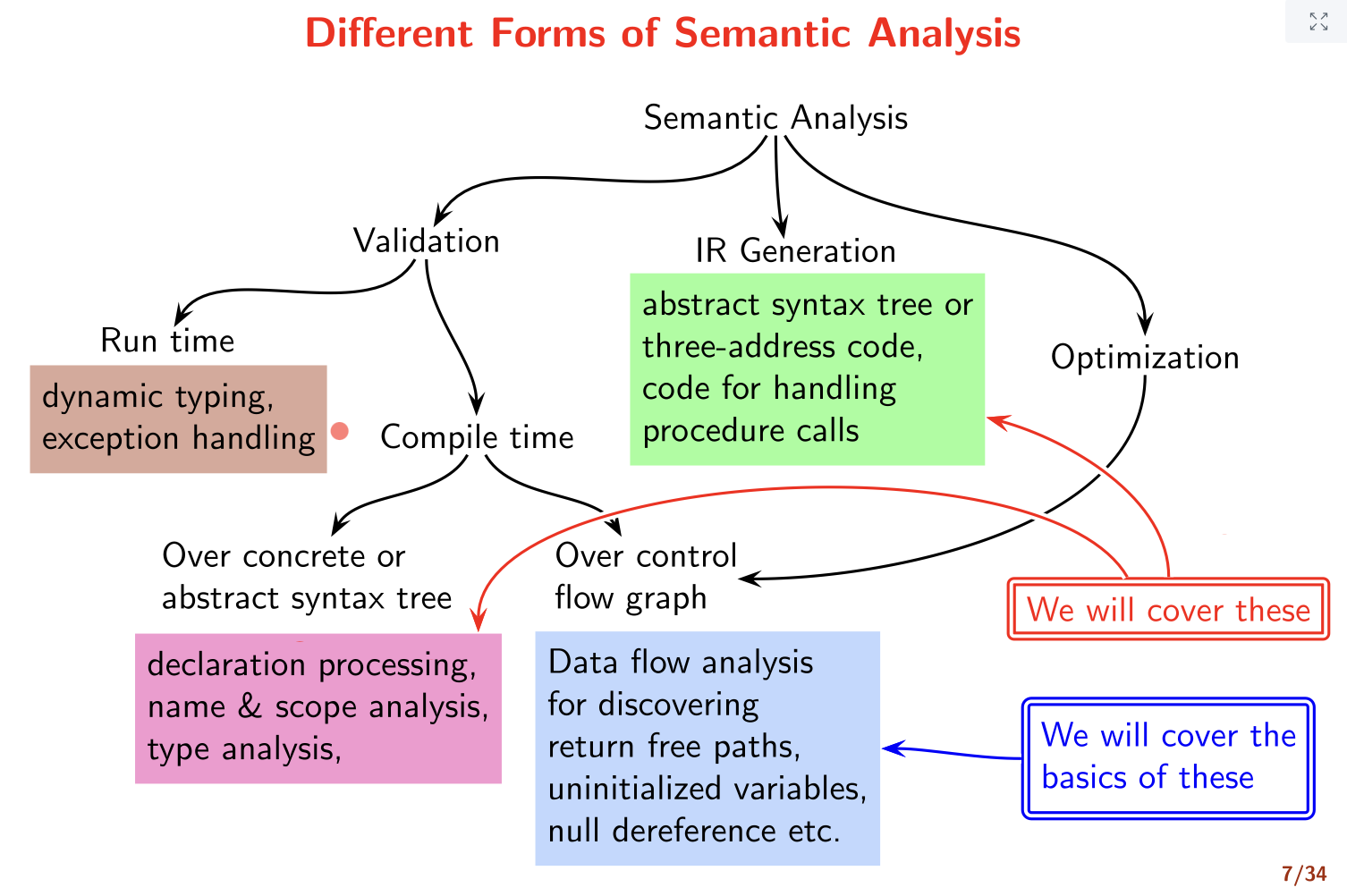
-
We have seen lexical errors and syntax errors. Name and scope analysis cannot be done using scanner and parser (as our grammar is context free). These are detected by semantic analyser and are known as semantic errors.
Compilers usually try to list all the errors in the program by trying to recover from each error, and continue compiling the remaining code.
- C++ requires references to be initialised.
-
Overflow shows up as a warning and not as an error. Why? This is because type conversions are allowed in C++. These sort of errors are runtime errors.
-
Suppose we have the following program
int i = 40;

cout<< 1 <= i <= 5 <<endl;
The output of this code is
1and not0. This is because1 <= iis evaluated asTrue(1) and1 <= 5isTrue.This is a runtime activity and the error cannot be identified by a compiler (unless constant propagation optimisation is performed). This error is known as a logical error.
Runtime and Logical errors are usually not detected by the compiler.
-
Does
int a[3] = {1, 2, 3, 4};give an error? Yes! (Too many initialisers) It’s a semantic error. What if we hadint a[4] = {1, 2, 3};cout<<a[3];? It does not give an error or a warning. It gives a runtime error in the form of a segmentation fault. -
Suppose we had the following code
int f(int a)
{
	if (a > 5) return 0;
}
Does this give an error? No, the compiler gives a warning that says “control reaches end of non-void function.” Such functions can be used to generate pseudorandom numbers. However, does
f(-5)give a runtime error? No, it returns-5. Why is that so?Also, if the definition of
fwas modified to the following, then we get random numbersint f(int a) { if (a > 5) return 0; cout << a << endl; }But again, if
fis modified to below, we start getting-5everytime.int f(int a) { if (a > 5) return 0; cout << a << endl; a = a + 5; } // Or the following f int f(int a) { if (a > 5) return 0; g(a); }Many such variations are possible with different behaviours. Also, the output of the program depends on the compiler flags too!
The language specifications say that a variable must be declared before its use but may not be defined before its use.
-
Consider the following code
float inc = 0.1, sum = 0;
while (inc != 1.0)
{
	sum += inc;
	inc += 0.1;
}
This program can go into an infinite loop due to floating imprecision. This is a runtime activity and cannot be detected by a compiler. We will classify this as a logical error and not a runtime error. Remember that
0does not cause any imprecision! -
Consider the following code
void f(short a) {cout<<"short";}
void f(long a) {cout<<"long";}
void f(char a) {cout<<"char";}
int main ()
{
	f(100);
}
How does the compiler decide which function to use? There is a difficulty in resolving function overloading. This is a semantic error. If we had a definition for
int, then there would not be any issue, as integer is a default type.Also, comparison of string and integer will give a syntax error.
-
mainin C can be recursive!
Lecture 13
02-03-22
Why separate semantic analysis from syntax analysis?
The constraints that define semantic validity cannot be described by context free grammars. Also, using context sensitive grammars for parsing is expensive. Practical compilers use CFGs to admit a superset of valid sentences and prune out invalid sentences by imposing context sensitive restrictions. For example, \(\{wcw \mid w \in \Sigma^*\}\) is not a CFG. We accept all sentences in \(\{xcy \mid x, y \in \Sigma^*\}\), enter \(x\) in a symbol table during declaration processing, and when ‘variable uses’ are processed, lookup the symbol table and check if \(y = x\).
We identify some attributes of the context-free grammar, and apply some constraints on them to simulate context-sensitivity.
Terminology
- Undefined behaviour - Unchecked prohibited behaviour flagged by the language. These are not a responsibility of the compiler or its run time support. They have unpredictable outcomes, and the compiler is legally free to do anything. Practical compilers try to detect these and issue warnings (not errors).
- Unspecified behaviour (aka implementation-defined behaviour) - These refer to a valid feature whose implementation is left to the compiler. The available choices do no affect the result by mat influence the efficiency. For example, the order of evaluation of subexpressions is chosen by the compiler. Practical compilers make choices based on well defined criteria,
- Exceptions - Prohibited behaviour checked by the runtime support. Practical compilers try to detect these at compile time.
Different forms of Semantic Analysis
Syntax Directed Definitions (SDDs)
The augmented CFG with attributes is given by
| \(A \to \alpha\) | \(b = f(c_1, c_2, \dots, c_k)\) | | —————– | ——————————- |
where \(b\) is an attribute of \(A\) and \(c_i\), \(1 \leq i \leq k\) are attributes of \(\alpha\). These semantic rules are evaluated when the corresponding grammar tules is use for derivation/reduction.
Note. The associativity decision is not decided through the order of execution, but through the order in which variables are ‘seen’.
Lecture 14
04-03-22
SDD for generating IR for expression
For example, consider the input statement \(x = (a - b) * ( c+ d)\). The expected IR output is
t0 = a - b
t1 = c + d
t2 = t0 * t1
x = t2
To achieve this, we can have a “code” attribute for each id, and then concatenate the codes to obtain the IR.
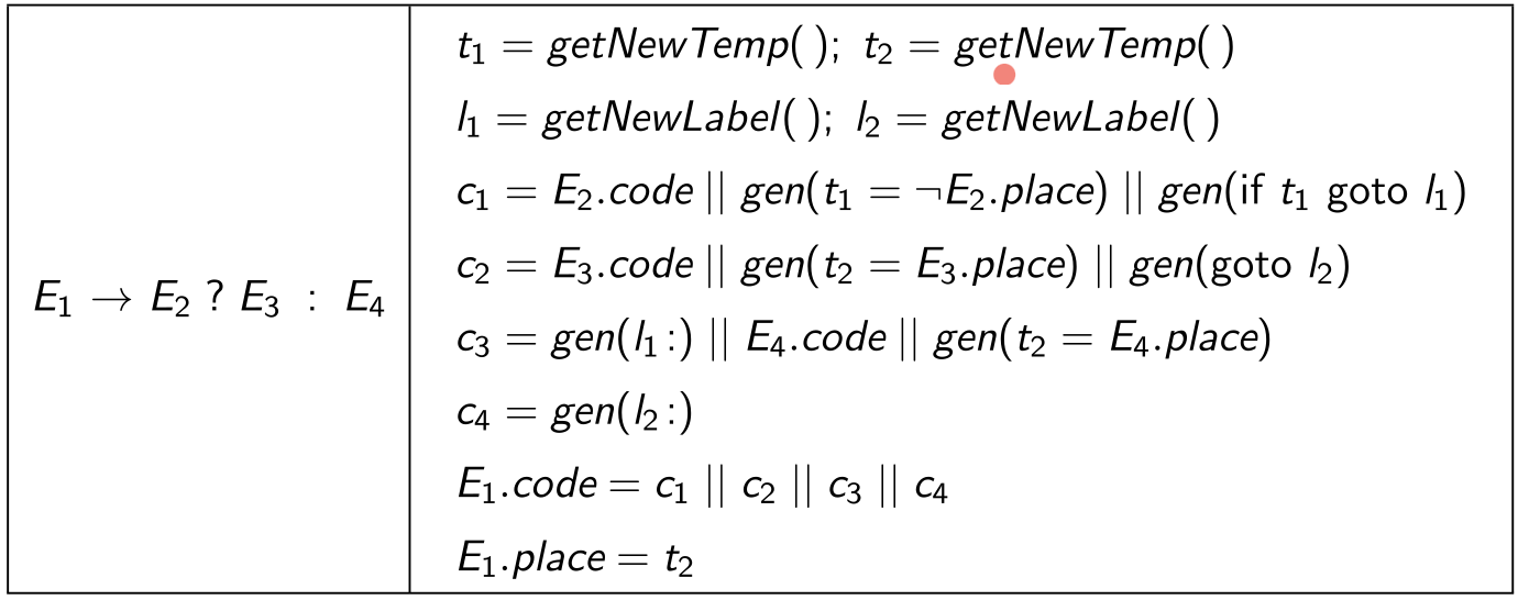
Let us consider the example for generating an IR for a ternary expression. We have \(E_1 \to E_2\ ?\ E_3 : E_4\). Then, we have the following template for the code of \(E_1\).
E_2.code
t_1 = !E_2.place
if t_1 goto I_1
E_3.code
t_2 = E_3.place
goto I_2
I_1 : E_4.code
			t_2 = E_4.place
I_2 :
--------------------------
E_1.place = t_2
Why are we using
!t1instead oft1? It is just a design decision.
Now, we shall use the following SDD for generating the above code.
There are two representations of a 2D array - row major representation and column major representation. FORTRAN uses column major representation for arrays.
Should the compiler decide the representation or should the language do it? Languages specify the representation!
In general, we use row-major representation where the address of the cell \((i, j)\) is given by base + i1*n2 + i2. For a general \(k\)-D array, the offset is given by the recurrence
We add the attributes name, offset, ndim etc for IR of array accesses.
Check the slides for the pseudocode to generate IR for unary/binary expressions, while loop etc.
Lecture 15
09-03-22
Generating IR for Field Accesses in a Structure
The ‘access’ expressions become a little more non-trivial in case of structures as compared to variables. The memory offsets of a structure can be computed at compile time unlike an array offset. For example, the offset in A[x] cannot be calculated at compile time. Hence, it is easier to work on structures. A float is considered to occupy 8 bytes.
The general IR code will have the following steps
- Obtain the base address
- Add the offset to the base
- Dereference the resulting address
We will assume offset(t, f) gives the offset of field f in structure t. Similarly, type(t, f) gives the type of f in t. The TAC generation code is given by
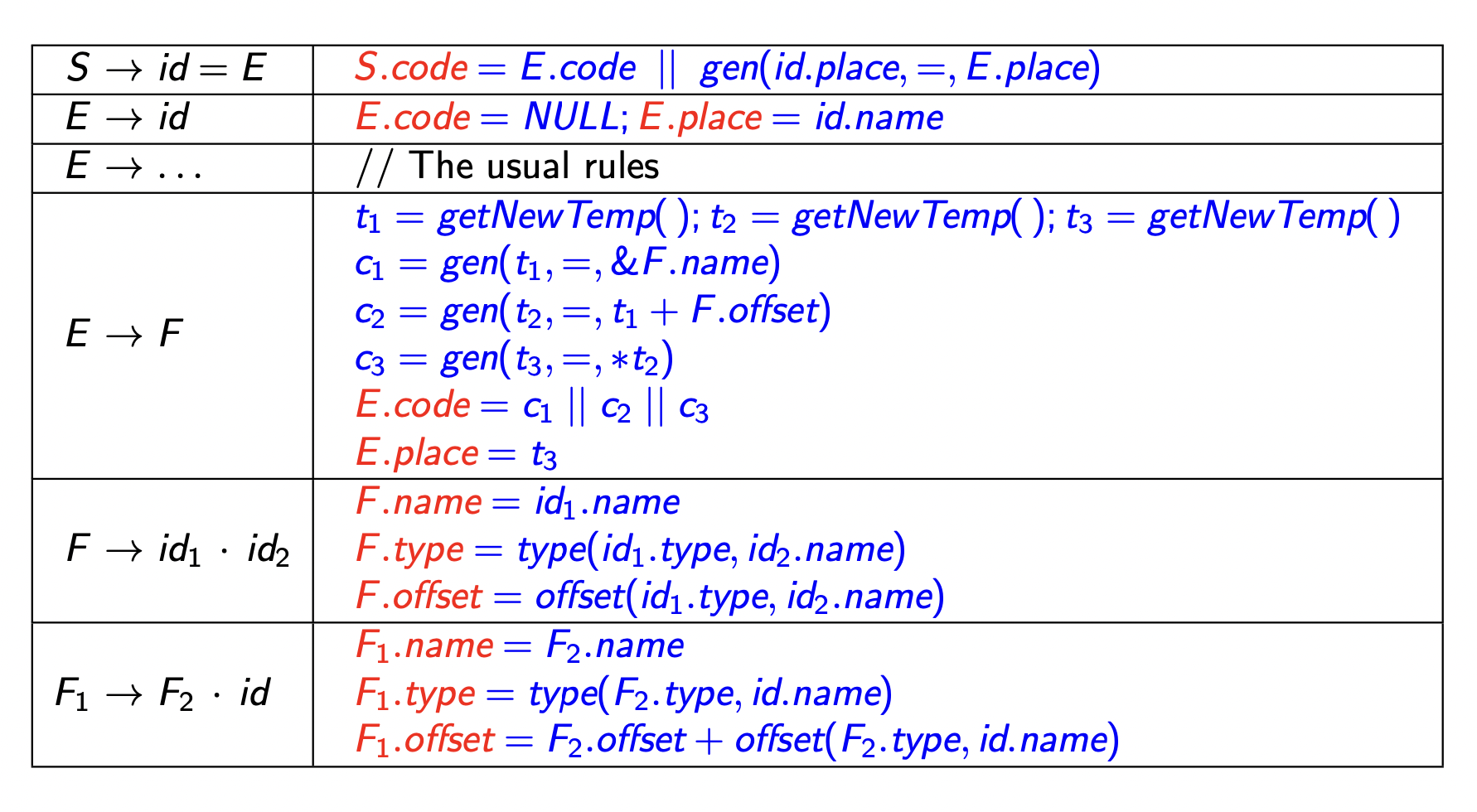
We need to add the code and place attributes to the above rules. We shall assume that the members of a class are stored sequentially based on the declaration.
Note. We cannot have a circular dependancy among classes without pointers.
We shall introduce pointers in our grammar now.
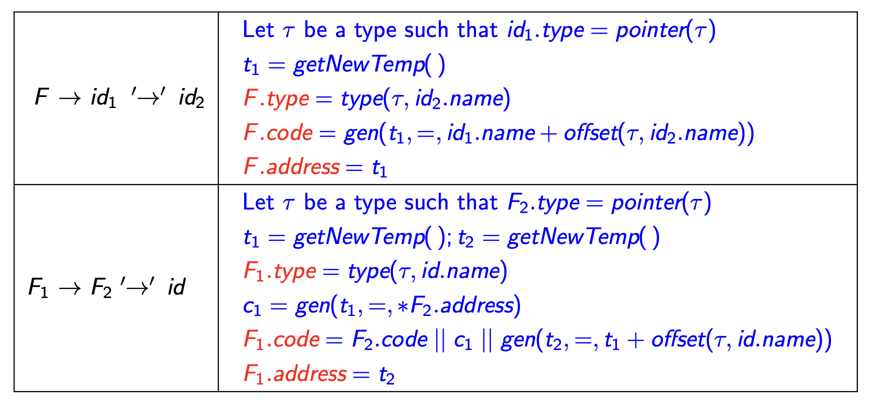
Note. The new code for \(F \to id_1.id_2\) generates different code as compared to our previous implementation.
Syntax Directed Translation Schemes
Given a production \(X \to Y_1Y_2 \dots Y_k\),
- If an attribute \(X.a\) is computed from those of \(Y_i\), \(1 \leq i \leq k\), the \(X.a\) is a synthesised attribute.
- If an attribute \(Y_i.a\), \(1 \leq i \leq k\) is computed from those of \(X\) or \(Y_j\), \(1 \leq j \leq i\), then \(Y_i.a\) is an inherited attribute.
Using these definitions, we will come up with an alternate approach for generating the IR for structures that is more expressive.
Lecture 16
11-03-22
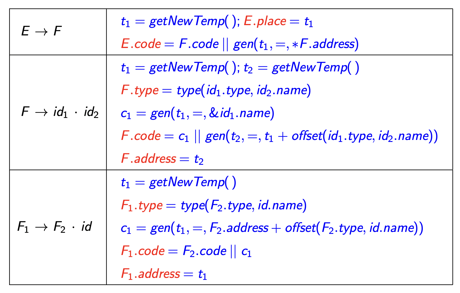
Previously, we had calculated the cumulative offset for a structure access in the IR. As in, we computed the final offsets at compile time and consequently used F.offset attribute instead of the F.code attribute. Alternately, we did not do ‘compile time offset calculation’ for the pointer IR code.
Let us now continue the discussion on inherited and synthesised attributes. A synthesised attribute is an attribute derived for a non-terminal on the lhs of a production from the non-terminals on the rhs of the same production. Inherited attributes are derived for non-terminals on the rhs of a production from the non-terminal on the rhs or other non-terminals on the rhs. So, why do we require inherited attributes?
For example, consider type analysis
Decl -> Type VarList {$2 -> type = $1 -> name}
Type -> int | float {$$ -> name = $2;}
VarList -> VarList, id {$1 -> type = $$ -> type; $3 -> type = $$ -> type;}
Varlist -> id {$1 -> type = $$ -> type;}
Here, the attribute type is inherited.
However, how do we allow flow of attributes concurrently with parsing? Clearly, there would be non-terminals that are not generated at a given step during parsing, and inherited attributes cannot be computed if they depend on a symbol not yet seen. All these problems can be avoided by no allowing inherited attributes to be derived from the symbols to the right of the current symbol. So once the left non-terminals are derived, we can derive the attribute for the current non-terminal.
In summary, given a production \(X \to Y_1, \dots, Y_k\)
- \(Y_i.a\) is computed only from the attributes of \(X\) or \(Y_j\), \(j < i\).
- \(X.a\) would have been computed from the grammar symbols that have already been seen (i.e, in some production of the form \(Z \to \alpha X\beta\))
More definitions
An SDD is S-attributed if it uses only synthesised attributes, and an SDD is L-attributed if it uses synthesised attributes or inherited attributes that depend on some symbol to the left. That is, given a production \(X \to Y_1\dots Y_k\) attribute \(Y_i.a\), of some \(Y_i\) is computed only from the attributes of \(X\) or\(Y_j\), \(j < i\).
Syntax Directed Translation Schemes (SDTS)
We generalise the notion of SDDs using SDTS. A Syntax Directed Translation Scheme is an SDD with the following modifications
- Semantic rules are replaced by actions possibly with side effects.
- The exact time of the action is specified; an action computing an inherited attribute of a non-terminal appears just before the non-terminal.
For example, for the previous type analysis rules, we have
decl -> type {$2 -> type = $1 -> type } VarList
We similarly define S-Attributed SDTS as SDTS that only use synthesised attributes and all actions appear at the end of the RHS of a production. L-Attributed SDTS use only synthesises attributes or attributes that depend on a symbol towards the left. The actions may appear in the middle of the rules end and at the end of the RHS of a production.
Type Analysis
Type Expressions and Representation
A type expression describes types of all entities (variable, functions) in a program - basic types, user-defined types, and derived types.
Note. The size of an array is not a part of the type in C for validation. It is just used for memory allocation. \(\tau_1 \times \tau_2\) describes the product of two types, and \(\tau_1 \to \tau_2\) describes a function that takes arguments described by \(\tau_1\) and returns the result described by \(\tau_2\). Product is left-associative and has a higher precedence than \(\to\).
Lecture 17
16-03-22
Marker Non-terminals
If we have a rule of the form \(X \to Y_1 \{\dots\} Y_2\), then we convert it to the following set of rules \(X \to Y_1 M Y_2 \\ M \to \epsilon \{\dots\}\) \(M\) is a marker non-terminal for \(Y_2\) in the grammar. \(Y_1.s\) and \(Y_2.s\) denote the synthesised attributes of \(Y_1\) and \(Y_2\) whereas \(Y_2.i\) denotes the inherited attribute of \(Y_2\).
When \(M \to \epsilon \{\dots\}\) is about to be reduced, the parsing stack contains \(Y_1\), and the value stack contains \(Y_1.s\). Once the reduction is done, we add \(M\) to the parsing stack, and \(Y_2.i\) is added to the value stack.
Marker non-terminals may cause reduce-reduce conflicts. It is possible to rewrite the yacc scripts to prevent these conflicts.
Type Analysis (2)
Type Equivalence
Consider two different with identical member variables and functions. How do we distinguish the structures themselves and pointers to these structures?
Name Equivalence - Same basic types are name equivalent. Derived type are name equivalent if they have the same name. every occurrence of a derived type in declarations is given a unique name.
Structure Equivalence - Same basic types are structurally equivalent. Derived types are structurally equivalent if they are obtained by applying the same type constructors to structurally equivalent types, or one is type name that denotes the other type expressions?.
Name equivalence implies structural equivalence and not the other way around. C uses structural equivalence for everything except structures. For structures, it uses name equivalence.
Type Inferencing
Functional languages do not require separate declarations for variables and types. Some sort of type inferencing is done for class during runtime in C.
Name and Scope Analysis
We maintain a stack of symbol tables. At the start of a new scope, we push a new symbol table on the stack. We start with the “global” scope symbol table. At the end of every scope, we pop the top symbol table from the stack. For use of a name, we look it up in the symbol table starting from the stack top
- If the name is not found in a symbol table, search in the symbol table below
- If the same name appears in two symbol tables, the one closer to the top hides the one below
However, with this setup, how do we access variables in the outer scope?
Static and Dynamic Scoping
Under static scoping/ lexical scoping, the names visible at line \(i\) in procedure \(X\) are
- Names declared locally within \(X\) before line \(i\)
- Name declared in procedures enclosing \(X\) upto the declaration of \(X\) in the program.
Under dynamic scoping, the names visible at line \(i\) in a procedure \(X\) are
- Names declared locally within \(X\) before line \(i\)
- Name declared in procedures enclosing \(X\) in a call chain reaching \(X\).
Dynamic scoping is difficult to comprehend is seldom used.
Lecture 18
23-03-22
Declaration Processing
How do we process int **a[20][10]? Do we take it as double pointer to an array of 20 rows where each row consists of 10 integers, or do we take it as a 2D-array of double arrays to integers with size \(20 \times 10\)?
In order to do the former, we can use the following grammar
\[\begin{align} decl &\to T \ item; \\ T &\to int \mid double \\ item &\to id \mid item [num] \end{align}\]However, this is an inconvenient layout for 20 arrays of arrays of 10 ints. Suppose we correct it to the following
\[\begin{align} decl &\to T \ item; \\ T &\to int \mid double \\ item &\to id \mid Array \\ Array &\to [num] \mid [num]Array \end{align}\]So basically, we have changed left recursive rule to a right recursive rule.
We introduce the notion of base types and derived types for We similarly add the size and width attributes in the above rules.
Addition of pointers is easy. We just add the following set of rules to the above set.
\[\begin{align} item &\to * \{item2.bt = item.bt\} \\ &\to item2 \\ &\to \{item.dt = pointer(item2.dt); item.s = 4\} \end{align}x\]Lecture 19
25-03-22
Runtime support
The data objects come into existence during the execution of the program. The generated code must refer to the data objects using their addresses, which must be decided during compilation.
Runtime support also helps in dynamic memory allocation, garbage collection, exception handling, and virtual function resolution.
Virtual function resolution falls under the category of runtime support as pointer declarations are static but the objects pointed are dynamic.
A programmer specifies the type of a data item, and also its role and allocation. Unnamed data resides on heap. We have the following properties of data
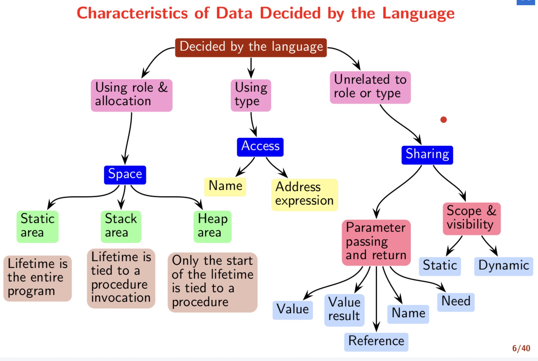
Local and global static variables?
A sequential language may allow procedures to be
- Invoked as subroutines - Stack and static memory suffices for organising data for procedure invocations.
- Invoked recursively - Stack memory is required for organising data for procedure invocations.
- Invoked indirectly through a function pointer or passed as a parameter. Access to non-local data of the procedure needs to be provided.
Compiling Procedure Calls
Activation Records
Every invocation of a procedure requires creating an activation record. An activation record provides space for
- Local variables
- Parameters
- Saved registers
- Return value
- Return address
- Pointers to activation records of the calling procedures
We maintain two parameters known as frame pointer and stack pointer. Activation record of the callee is partially generated by the caller. We store the return parameter in one of the registers itself. Function prologue and function epilogue are generated by the compiler. We reduce the value of stack pointer when we push something on the stack. The stack pointer $sp points to the lower address of the next free location. Unlike the stack pointer, the frame pointer $fp holds the address of an occupied word.
Reminder. We are talking about runtime activity.
As discussed earlier, the compiler generates a function prologue and epilogue. It also generates a code before the call and after the call. This is all the boring assembly code we typically see for calling functions. We shall this code changes when the parameter passing mechanism changes. We will also see implicit sharing through scoping.
Lecture 20
30-03-22
Using Static/Access Link
Let us reiterate the difference between static and dynamic scoping. In static scoping, we can use variables that are declared in the outer scope of the current scope. We use static/access link for this purpose. On the other hand, dynamic scoping follows the call chain for variables. We use control/dynamic link for this purpose.
To access the activation record of a procedure at level \(l_1\) from within a procedure at level \(l_2\), we traverse the access link \(l_2 - l_1\) times. Note that \(d_{callee} \leq d_{caller}+ 1\).
Parameter Passing Mechanisms
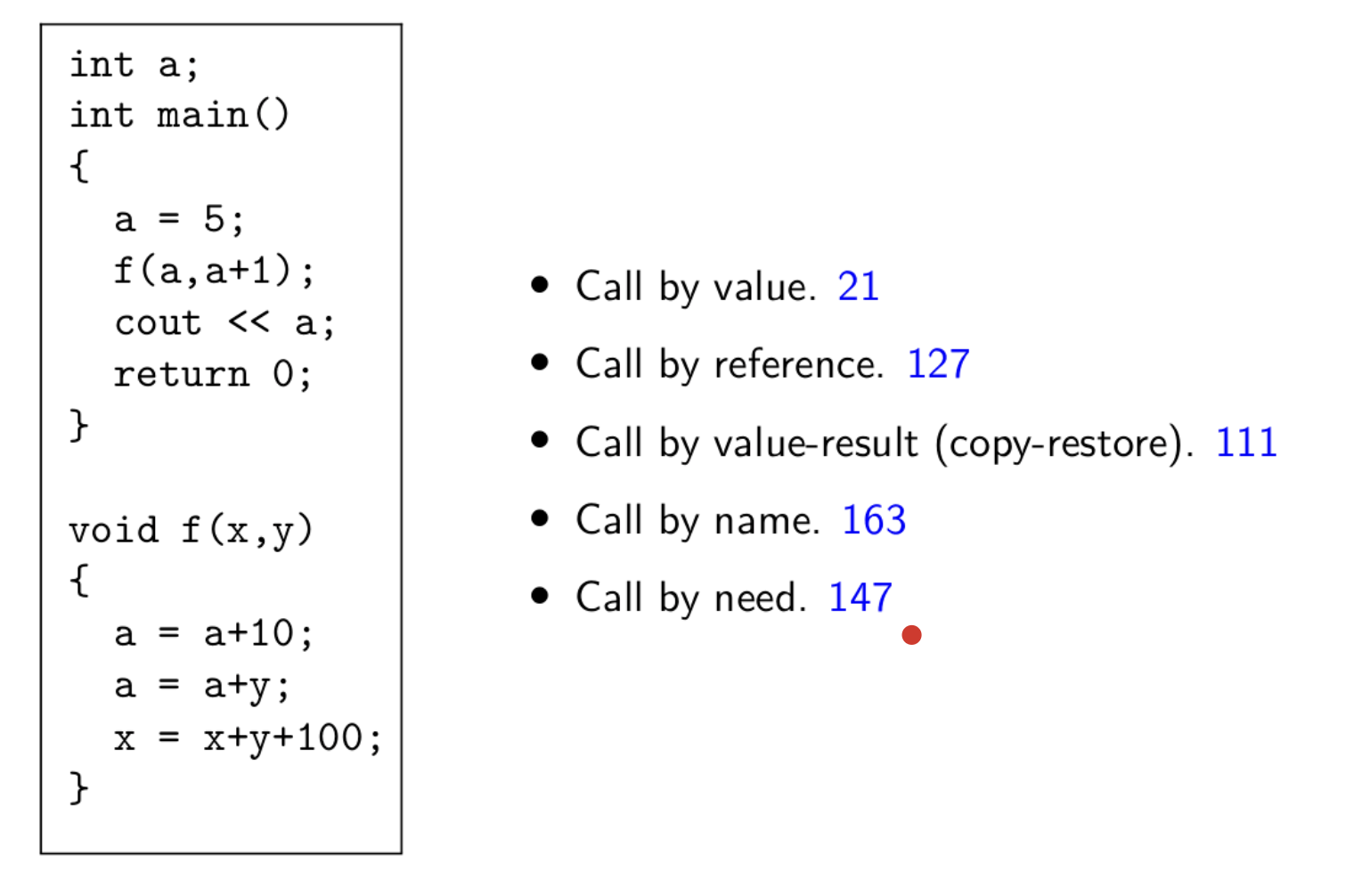
- Call by value - Copy the value of the actual parameter into the formal parameter. We use eager evaluation here. We do not know if the parameter is being used in the procedure, but we still evaluate it.
- Call by reference - Copy the address of the actual parameter into the formal parameter.
- Call by value-result (copy-restore) - Copy the value of the actual parameter and copy the final value of the formal parameter into the actual parameter. This method starts off with call by value. That is, the value of the actual parameter is copied into the formal parameter. However, in the end the value of the formal parameter that is evaluated inside the procedure is copied to the actual parameter. In the end we do
*(&e) = xand note = xbecauseeis an expression. - Call by name - Textural substitution of formal parameter by the actual parameter. Evaluation of the actual parameter is delayed until the value of formal parameter is used. The evaluation is done every time where the formal parameter is used in the procedure. So, this is equivalent to textual substitution or using a macro. All the modifications to the formal parameter is written to the address of the actual parameter. This is implemented by a thunk which is a parameterless procedure per actual argument to evaluate the expression and return the address of the evaluation.ccc
- Call by need - Textual substitution of formal parameter by the actual parameter but evaluation only once. This is similar to call by name but the evaluation of the actual parameter is done only at the first use. For any later use, we use the precomputed values. This is known as lazy evaluation.
We have the above to make the distinction between the different methods.
Parameter Passing Mechanisms for Procedure as Parameters
Pass a closure of the procedure to be passed as parameter. A data structure containing a pair consisting of
-
A pointer to the procedure body
-
A pointer to the external environment (i.e. the declarations of the non-local variables visible in the procedure)
Depends on the scope rules (i.e., static or dynamic scope)
For C, there are no nested procedures so the environment is trivially global. So a closure is represented trivially by a function pointer. In C++, the environment of a class method consists of global declarations and the data members of the class. The environment can be identified from the class name of the receiver object of the method call.
Representation of a Class
There is no distinction between the public and private data in memory. Public/Private is a compile time distinction. Every function with \(n\) parameters is converted to a function of \(n + 1\) parameter with the first parameter being the address the address of the object. Internally, the data space is separate for each object, but the code memory is same for all which contains the functions.
Virtual functions
Non-virtual functions are inherited much like data members. There is a single class-wide copy of the code and the address of the object is the first parameter as seen earlier. In the case of virtual functions, a pointer to a base class object may point to an object of any derived class in the class hierarchy.
Virtual function resolution
Partially static and partially dynamic activity. At compile time, a compiler creates a virtual function table for each class. At runtime, a pointer may point to an object of any derived class, and the compiler-generated code is used to pick up the appropriate function by indexing into the virtual table for each class.
We define a non-virtual function as a function which is not virtual in any class in a hierarchy. Resolution of virtual functions depends on the class of the pointee object - needs dynamic information. Resolution of non-virtual functions depends on the class of the pointer - compile time information is sufficient. In either case, a pointee cannot belong to a “higher” class in the hierarchy.
Lecture 21
01-04-22
Compiler decides the virtual function for a class statically. Functions are not copied across objects but are used with reference. Functions of the inherited class override the corresponding virtual functions of the parent class. There is no search for the correct function implementation during the runtime. Instead, all the functions are correctly configured at compile time.
The runtime support looks up the class of the receiver object. Then, it dereferences the class information to access the virtual function table. Following this, there is another dereference to invoke the function itself.
Note. A pointer of the parent class can hold an object of the inherited class but not the other way around. However, when the pointer for the parent class is used, the functions in the inherited class that are not present in the parent class cannot be invoked. That is, the pointer will only be able to invoke functions from the parent class.
Note. Functions of the parent class can be overridden without using virtual functions. Non-virtual functions are copied in each class. However, pointer references are used in the case of virtual functions. In the case of virtual functions, the pointer of the base class holding an inherited class object will call the functions of the inherited class and not the base class.
For example, consider the following
class A {
public:
        virtual int f() { return 1; }
        int g() {return 2};
};

class B : public A {
public:
        int f() { return 10; }
        int g() { return 20; }
};
...
A* p; B b;
cout << p -> f(); // Prints 10
cout << p -> g(); // Prints 2
Where are all the unique implementations of virtual functions stored?
Optimisations
Register Allocation
Accessing values from the registers in much faster than from the cache.
Glocal register allocation using Graph Coloring
We identify the live ranges for each variable, and then construct an interference graph between variables if there is any overlap in the live ranges. Then, we use graph coloring to register allocation. However, graph coloring with \(k\) colors is NP-complete general. We use some heuristics, and we shall study one of them called - Chaitin-Briggs allocator. The problem is decidable for chordal graphs - Every cycle of length 4 or more has a chord connecting two nodes with an edge that is not part of the cycle (applies recursively). Most practical interference graphs are chordal.
Chaitin-Briggs Register Allocator
-
Coalescing
We eliminate copy statements
x = yso that we use the sam register for both the variables. Then, the copy propagation optimisation replaces the used ofxbyy. -
Identification of live ranges
It is the sequences of statements from a definition of a variable to its last use of that values. We shall discuss live variables analysis later.
-
Identification of interference and construction of interference graph
Live ranges \(I_1\) and \(I_2\)
-
Simplification of interferences graph to identify the order in which the nodes should be colored.
Copy Propagation Optimisation
We assume intra-procedural lines of code. That is, the parts of code without any function calls.
Slides - Why
e3and note? The number3represents the statement number whereewas generated.
Discovering Live Ranges
Live ranges are calculated by traversing the code from the end to the beginning. We depict the live range as a set of statement indices. Then we check set intersection for interferences.
Lecture 22
06-04-22
Following the analysis of live ranges, we construct the interference graph. Along with the degree of each node, we note the number of loads and stores of each variable. We define spill cost as the sum of loads and stores for each variable.
Chaitin-Briggs Allocator
Let \(k\) be the number of colors. We discuss Chaitin’s method first.
-
We simplify the graph by removing the nodes in an arbitrary order such that for each node \(n\), \(D(n) < k\) and push them no a stack. Since \(D(n) < k\), we are guaranteed to find a color for \(n\).
How to prove?
-
If the graph is not empty, we find the node with the lease spill cost, and then we spill it. That is, we further simplify the graph by removing nodes with the lowest spill cost. Then, we repeat the first step.
-
Now, after all the simplification is done, we repeatedly pop the node from the top of the stack, plug it in the graph and give it a color distinct from its neighbour.
Now, let us see Briggs’ method
- Same as that of Chaitin’s method.
- Briggs’ conjectured that it is not necessary for all nodes with a degree greater than \(n\) not to have a color in the coloring. So, we mark the nodes as potentially spill-able and stack them.
- As in Chaitin’s method, we repeatedly color the nodes. If a node cannot be colored, we spill it and go back to the first step.
Spilling Decisions
-
Spill cost is weighted by loop nesting depth
\[C(n) = (L(n) + D(n)) \times 10^d\] -
Sometimes, we normalise \(C(n)\) and consider \(C(n)/D(n)\).
Chaitin’s method cannot color the square/diamond graph with 2 colors whereas Briggs’ method can.
Note. We consider the degree of nodes in the original graph. That is, when we simplify the graph in step 1, we don’t update the degrees of all the nodes at each iteration.
Allocating registers
Once we allocate the colors, we replace each variable by a register corresponding to a color. After replacing the code with registers, there would be redundant statements like r4 = r4. We can get rid of such statements, and this is known as Peephole Optimisation. (This happens due to control transfer)
Live range spilling
Spilling a live range \(l\) involves keep the variable of \(l\) in the memory. For RISC architecture, load in a register for every read, store back in the memory for every write. For CISC architectures, we access directly from the memory.
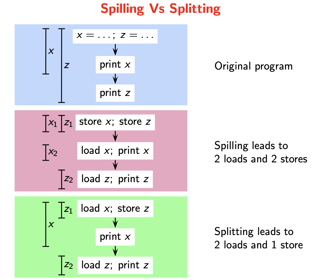
Spilling is necessary if the number of interfering live ranges at a program point exceeds the number of registers. Flow sensitivity (interval interferes with, say, 1 interval at any given time) vs Flow insensitivity (total number of overlaps is greater than 1).
Splitting a live range \(l\) involves creating smaller live ranges \(l_1, \dots, l_k\) such that \(D(l_i) \leq D(l), 1 \leq i \leq k\). Live ranges \(l_i\) can participate in graph coloring if \(D(l_i) < D(l)\). Therefore, we have a choice between splitting and spilling. The difference between the two approaches is shown here.
Registers across Calls
So far, we have seen allocation of local registers. Suppose we have the following situation. A function g() uses a register r and calls f() inside its body. Now, how do we manage r across the call?
- Procedure
gsaves it before the call and restores it after the call. However,g()does not know iff()requiresr. Here, save and restore is redundant iffdoes not requirer, and this is unavoidable. Also, it knows if the value inris need after the call. Here, save and restore is redundant ifris not required across the call, and this is avoidable. - Procedure
fsaves it at the start and restores it at the end. Now,fdoes not know ifgusesrafter the call, but it knows ifris required inf. Like before, the first problem is unavoidable but the second one is avoidable.
Now, as both methods are functionally similar, the method used is a matter of convention. The architecture decides this for the system. So, we have
- Caller-saved register - Callee can use it without the fear of overwriting useful data
- Callee-saved register - Caller can use it without the fear of overwriting useful data.
We use a caller-saved register r for values that are not live across a call. Then, r is not saved by the callee and need not be saved by the caller. We use a callee-saved register r for values that are live across a call. r is not saved by the caller, and it is saved by the callee only if it is needed.
Integrating with graph coloring
To begin with, the live range of a callee saved register is the entire procedure body of g, and the live range of a caller saved register is the procedure body of f. We then construct the interference graphs with these additional live ranges.
Lecture 23
08-04-22
Instruction Selection
We need to generate an assembly code from the “register code” we generated after register allocation. Floating point comparison takes 2 arguments whereas integer comparison takes 3 arguments.
Integrated Instruction Selection and Register Allocation Algorithms
- Sethi-Ullman Algorithm - Used in simple machine models, and is optimal in terms of the number of instructions with the minimum number of registers and minimum number of stores. It is also linear in the size of the expression tree.
- Aho-Johnson Algorithm - This algorithm is applicable for a very general machine model, and is optimal in terms of the cost of execution. It is also linear in the size of the expression tree (exponential in the arity of instruction which is bounded by a small constant). The main motivation behind this idea is that a sequence of 4 instructions can be more efficient than 2 instructions.
Sethi-Ullman Algorithm
WE have a finite set of registers \(r_0, \dots, r_k\) and countable memory locations. We will be using simple machine instructions like loads, store, and computation instructions (\(r_1 \; op \; k\), \(k\) can be a register or a memory location). The input to this algorithm is the expression tree (essentially the AST) without
- control flow (no ternary expressions)
- assignments to source variables inside an expression (so no side effects). Assignments are outside the expression.
- no function calls
- no sharing of values (trees, not DAGs). For example, we don’t have expressions like \(b \times c + d - b \times c\). Basically, we shouldn’t use common subexpression elimination.
The key idea behind this algorithm is that the order of evaluation matters. Sometimes, the result is independent of the order of evaluation of some subtrees in the tree. For example, in \(b \times c + a /d\), the order of evaluation of \(b \times c\) and \(a/d\) does not matter.
Therefore, we choose the order of evaluation that minimises the number of registers so that we don’t store an intermediate result in the memory.
In the algorithm, we traverse the expression tree bottom up and label each node with the minimum number of registers needed to evaluate the subexpression rooted at the node. Then, we traverse the tree top down and generate the code. Suppose we have
				op
			/    \
		l1      l2
Assume \(l_1 < l_2\). If we evaluate the left subtree first, we need \(l_1\) registers to evaluate it, 1 register to hold its result and \(l_2\) registers to evaluate the right subtree. Therefore, the total registers used would be \(\max(l_1, l_2 + 1)\) = \(l_2 + 1\). If we follow the other order, we get the number of registers as \(\max(l_2, l_1 + 1) = l_2\). Therefore, we evaluate the subtree with larger requirements first. So, we have the following recursion
\[label(n) = \begin{cases} 1 & n \text{ is a leaf and must be in a register n or it is a left child} \\ 0 & n \text{ is a leaf and can be in memory or it is a right child} \\ max(label(n_1), label(n_2)) & n \text{ has two child nodes with unequal labels} \\ label(n_1) + 1 & n \text{ has two children with equal labels} \\ \end{cases}\]If we generalise to instructions and trees of higher arity, then for node \(n\) with \(k\) children we get
\[label(n) = \max(l_j + j - 1), 1 \leq j \leq k\]Note that the above algorithm generates a store free program. Why aren’t we interleaving the codes of two subtrees? There is a notion of contiguity. Also, we are assuming that memory does not add any additional overhead in terms of CPU cycles.
How do we generate the code for the tree? rstack is a stack of registers, and gencode(n) generates the code such that the result of the subtree rooted at \(n\) is contained in top(rstack). tstack is a stack of temporaries used when the algorithm runs out of registers. swap(rstack) swaps the two top registers in rstack. Finally, the procedure emit emits a single statement of the generated code.
Then, we have
| Cases | gencode(n) |
|---|---|
| \(n\) is a left leaf | emit(top(rstack) = name). This invariant that the top of the rstack is the result is maintained. |
| The right child of \(n\) is a leaf | emit(top(rstack) = top(rstack) op r.name) |
| \(l_1 \geq l_2\) for children \(l_1, l_2\) of \(n\) | gencode(n_1)R = pop(rstack)gencode(n_2)emit(R = R op top(rstack))push(R, rstack) |
| \(l_1 < l_2\) | swap(rstack)gencode(n_2)R = pop(rstack)gencode(n_1)emit(top(rstack) = top(rstack) op Rpush(R, rstack)swap(rstack) |
| Both children need more registers than available | gencode(n_2)T = pop(tstack)emit(T = top(rstack)gencode(n_1)emit(top(rstack) = top(rstack) op T)push(R, rstack) |
In the above, R can be seen as a local static variable of the procedure. In the last case, we evaluated the right child first because only the right child can be a memory argument.
Lecture 24
13-04-22
Analysis of Sethi-Ullman algorithm
The register usage in the code fragment for a tree rooted at \(n\) can be described by
- \(R(n)\) the number of registers used by the code
- \(L(n)\) the number of registers live after the code (the intermediate results that are required later)
- The algorithm minimises \(R(n)\) to avoid storing intermediate results.
If the code computes the left child \(n_1\) first then, \(R(n) = \max(R(n_1), L(n_1) + R(n_2))\) and vice versa for the right child \(n_2\). In order to minimise \(R(n)\), we minimise \(L(n_1)\) and \(L(n_2)\). How do we do that?
-
Contiguous Evaluation - We evaluate \(n_1\) completely before evaluating \(n_2\) or vice versa. The reason this minimises the registers is that when we evaluate a subtree completely, we need to hold only the final result in a register during the evaluation of the other subtrees. Otherwise, we may have to hold multiple intermediate results in a register during the evaluation of the other subtree.
-
Strongly Contiguous Evaluation All subtrees of the children are also evaluated contiguously.
In Sethi-Ullman algorithm, each node is processed exactly, and hence the algorithm is linear in the size of the tree. Also, recall that we always evaluate the lowermost subtrees first for optimisation as mentioned somewhere before.
Arguing the Optimality
We define a node \(n\) to be a
- dense node - if \(label(n) \geq k\)
- major node - if both of its children are dense. A major node falls in case 5 of the algorithm.
where \(k\) is the number of registers, and \(label\) refers to the number of registers required at this node. Note that every major node is dense but not vice-versa. The parent of every dense node is dense but the parent of every major node need not be major! Also, these categories are dynamic. That is, when we store a dense node, the parent of this node can cease to be a major node. The major nodes decrease by at most 1 when we store a node.
Now, the algorithm generates
- exactly one instruction per operator node
- exactly one load per left leaf
- no load for any right leaf
The algorithm is optimal with regards to these counts. The optimality now depends on not introducing extra stores. Consider an expression tree with \(m\) major nodes.
- A store can reduce the number of major nodes by at most one. This is because, the node that becomes non-major, still remains a dense node so its parents remain a major node.
- Hence, the tree would need at least \(m\) stores regardless of the algorithm used for generating code
- The algorithm generates a single store for every major node as part of Case 5, thus it generates exactly \(m\) stores
- Since this is the smallest number of stores possible, the algorithm is optimal.
Enjoy Reading This Article?
Here are some more articles you might like to read next: