Key Works in ML Systems
Acknowledging use of Perplexity, ChatGPT and the reference books and papers to aid with the content.
Introduction
As with every other article, this one starts with the same remark too - We are at an inflection point in human history. Artificial Intelligence (AI) is everywhere, and its growth has been unparalleled. We are in the AI revolution.
At times like these, it is important to think about the future - how do we create systems that work alongside humanity to tackle the biggest problems life faces? We must master a new field of engineering to maintain this unprecedented pace.
History of AI

Starting with symbolic AI, one of the early approaches, STUDENT system developed by Daniel Bobrow in 1964, demonstrated natural language understanding by converting English text into algebraic equations. However, it was a rule-based system that was very brittle to the grammatical structure - although the solution may appear intelligent, it did not have a genuine understanding of language or the actions it was taking. This issue is the primary problem behind rule-based approaches.
Then followed expert systems in 1970s, which focused on domain specific problems over generalized AI. For example, MYCIN developed by Stanford showed a major leap in medical AI with it’s 600 rules-based system. Nevertheless, scaling these rules with newer discoveries is infeasible.
Statistical Learning
In the 1990s, something radical happened - the field moved away from rules to data-driven approaches. With the digital revolution, new capabilities got unlocked. From regression to neural networks, we allowed machines to discover patterns in the data leading to diverse applications. This new paradigm changed the way we approached machine learning. Quality of data, metrics to evaluate performance and trade-offs in design choices - all became relevant research questions.
During the 2000s, algorithms like decision trees and KNNs made their way into practical applications. SVMs with their “kernel trick” became very popular. Human engineered features combined with statistical learning was the characteristic in the algorithms, and they had strong mathematical foundations as well. The models performed well with limited data, and produced reliable results. Even modalities like face detection with Viola-Jones algorithm (2001) became feasible.
Deep Learning
A double-edged sword, deep learning became the new kid in the block since the 2010s. Deep learning networks automatically discovered features in the data, doing away with feature engineering. Starting with AlexNet in 2012, the successes with deep learning models have never been shy. Researchers realized that bigger models equals better performance. Now, in the 2020s, we have entered the age of large models which have parameters reaching into few hundreds of billions! The datasets are well into the Petabytes stage.
The three pillars required for these models to be successful, big data, better compute, and algorithmic breakthroughs, have successfully been put in place over the past few decades.
These new depths have raised important questions about the future: how do we store and serve such models and datasets?!
ML Systems Engineering
It is the discipline of designing, implementing, and operating AI systems across computing scales. A machine learning system is an integrated computing system with three main parts - data, models and the compute infrastructure.
Software Engineering as a field has been well established over the past decade. Even though the field is not yet mature, it has practices in place to enable reliable development, testing and deployment of software systems. However, these ideas are not entirely applicable to Machine Learning systems. Changes in the data distribution can alter the system behavior - this is a new paradigm we have not addressed before.
More than often, the performance requirements guide the design decisions in the architecture. The complexities arise due to the broad spectrum across which ML is deployed today - from edge-devices to massive GPU-cloud clusters, each presents unique challenges and constraints. Operational complexities increase with system distribution. Some applications may have privacy requirements. The budget of the system acts as an important constraint. All these tradeoffs are rarely simple choices.
Modern ML systems must seamlessly connect with existing software, process diverse data sources, and operate across organizational boundaries, driving new approaches to system design. FarmBeats by Microsoft, Alphafold by Deepmind and Autonomous vehicles are excellent examples of how proper systems in place can really push the extent of ML applicability.
Challenges
-
Data Challenges - How do we store and process different kinds of data, and how to accommodate patterns with time?
-
Model Challenges - How do we create efficient systems for different forms of learning, and test their performance across a wide range of scenarios?
-
Systems Challenges - How do we set up pipelines in place to combine all of this in place? Systems that have monitoring and stats, that allow model updates and handle operational challenges.
-
Ethical and Social Considerations - How do we address bias in such large-scale models? Can we do something about the “black-box” nature? Can we handle data privacy and handle inference attacks?
A major solution to address all these challenges has been to democratize AI technology. Similar to an “all hands-on deck” solution, with the involvement of a large amount of people in this evolution, we are tackling one of the most innovative problem’s humanity has ever faced - how do we achieve AGI?
DNN Architectures
Assuming the reader’s know enough about different model architectures, we shall now discuss the core computations involved in these models to design the systems around them.
Architectural Building Blocks
So far, we have the following major architectures summarized below -
Multi-Layer Perceptrons (MLPs)
-
Purpose: Dense pattern processing
-
Structure: Fully connected layers
-
Key operation: Matrix multiplication
-
System implications:
- High memory bandwidth requirements
- Intensive computation needs
- Significant data movement
Convolutional Neural Networks (CNNs)
-
Purpose: Spatial pattern processing
-
Key innovations: Parameter sharing, local connectivity
-
Core operation: Convolution (implemented as matrix multiplication)
-
System implications:
- Efficient memory access patterns
- Specialized hardware support (e.g., tensor cores)
- Opportunity for data reuse
Recurrent Neural Networks (RNNs)
-
Purpose: Sequential pattern processing
-
Key feature: Maintenance of internal state
-
Core operation: Matrix multiplication with state update
-
System implications:
- Sequential processing challenges
- Memory hierarchy optimization for state management
- Variable-length input handling
Transformers and Attention Mechanisms
-
Purpose: Dynamic pattern processing
-
Key innovation: Self-attention mechanism
-
Core operations: Matrix multiplication and attention computation
-
System implications:
- High memory requirements
- Intensive computation for attention
- Complex data movement patterns
Some innovations like skip connections, normalization techniques, and gating mechanisms are highlighted as important building blocks that require specific architectures. With these in mind, we require the following primitives -
-
Core Computational Primitives -Matrix multiplication, Sliding window operations, Dynamic computation
-
Memory Access Primitives - Sequential access, Strided access, Random access
-
Data Movement Primitives - Broadcast, Scatter, Gather and Reduction
We address these primitives, by designing efficient systems as well as hardware.
-
Hardware - Development of specialized processing units (e.g., tensor cores), Complex memory hierarchies and high-bandwidth memory, Flexible interconnects for diverse data movement patterns
-
Software - Efficient matrix multiplication libraries, Data layout optimizations, Dynamic graph execution support
Conclusion
In summary, understanding the relationship between high-level architectural concepts is important for their implementation in computing systems. The future advancements in deep learning will likely stem from both novel architectural designs and innovative approaches to implementing and optimizing fundamental computational patterns.
Now that we have understood the basics of Machine Learning Systems, let us delve into the two biggest frameworks that support the ML systems today.
TensorFlow: A system for large-scale machine learning
A product of Google brain built to tackle large scale systems in heterogeneous environments. TensorFlow uses data-flow graphs to represent computations, shared states and operations. These can be mapped across many machines giving a flexibility to the developers.
TensorFlow is based on a previous product of Google Brain, DistChild, that was used for a large number of research and commercial tasks. The team recognized the recent advances in ML - CNNs that broke records reaching up to millions of parameters and GPUs that accelerated the training processes. They developed a framework that is well-optimized for general scenarios for both training and inference. They also meant for it to be extensible - to allow ability to experiment and scale in production with the same code.
Prior to this work, Caffe, Theano and Torch were the major frameworks. Caffe was known for its high-performance, Theano for its data flow model and Torch for its imperative programming model. Along with these works, TensorFlow also draws inspiration from the map-reduce paradigm that improved the performance of data systems significantly.
TensorFlow execution model
The computation and state of the algorithm, including the mathematical operations are represented in a single dataflow graph. The communications between the subcomputations are made explicitly to execute independent computations in parallel and partition the computation across distributed devices. The key point to note here is that the graph has mutable states for the individual vertices, meaning that data can be shared between different executions of the graph. Although this point may seem trivial now, architectures prior to TensorFlow worked with static computations graphs that did not allow changes to the weights - algorithms such as mini-batch gradient descent were not scalable to large parameter models. Due to this change in the architecture, developers can experiment with different optimization algorithms, consistency schemes and parallelization strategies.
Dataflow graph elements
Each vertex in the dataflow graph is an atomic unit of computation and each edge is the output or input to a vertex - values flowing through tensors.
Tensors - Notably, tensors as a computational quantity were introduced in this paper. Their work assumes all tensors are dense - this allows simple implementations for memory allocation and serialization.
Modern neural networks on the contrary have sparse tensors in many scenarios - can be optimized greatly
TensorFlow does allow representing sparse tensors but at the cost of more sophisticated shape inference.
Operations - An operation can simply be thought of as a function that takes \(m \geq 0\) tensors as input and returns \(n \geq 0\) tensors as output. The number of arguments to these operators can be constant or variable (variadic operators). Stateful operations (variables and queues) contain mutable states that can be updated every time the operator executes. Variables are mutable buffers storing shared parameters and queues support advanced forms of coordination.
Partial and concurrent execution
The key advantage of storing the dataflow as a graph is the ability to execute independent operations in parallel. Once a graph is defined by the user, the API allows for executing any sub-graph the user queries. Each invocation is a step and TensorFlow supports multiple concurrent steps. This ability shines for the batch-processing workflows in neural networks. Furthermore, TensorFlow has a checkpointing subgraph that runs periodically for fault tolerance.
This functionality of running graphs partially and concurrently contribute much to TensorFlow’s flexibility.
Distributed execution
Since the communication between subcomputations is explicit, the distribution of the dataflow becomes simpler. Each operation resides on a particular device (note that this feature has also been adapted in PyTorch), and a device is responsible for executing a kernel for each operation assigned to it. TensorFlow allows multiple kernels to be registered for a single operation.
The placement algorithm computes a feasible set of devices for each operation, calculates the sets of operations that must be colocated and selects a satisfying device for each colocation group. In addition, the users can also specify their device preferences for a particular task. Yes, TensorFlow was advanced since the beginning.
Once the operations are placed, the partial subgraphs are computed for a step, and are pruned and partitioned across the devices. The communication mechanisms between devices is also put in place with specialized implementations to optimize for latency with large-subgraphs running repeatedly. On the user-end, a client session maintains a mapping from step definitions to cached subgraphs. This computation model performs the best with static, reusable graphs but also supports dynamic computations with control flows.
Dynamic control flow
Although most evaluation in TensorFlow is strict, wherein it requires for all inputs to an operation to be computed before the operation executes, advanced algorithms (such as RNNs), require dynamic control flow, requiring non-strict evaluation. To aid with this, TensorFlow also supports primitive Switch (demultiplexer) and Merge (multiplexer) operations for dynamic dataflow architectures! These primitives can be used to build a non-strict conditional sub-graph that executes one of two branches based on the runtime values of a tensor. These primitives also support loops with additional structural constraints based on the dataflow!
Extensibility
-
Differentiation - TensorFlow has a user-level library that automatically differentiates expressions. It performs a breadth-first search to identify all of the backwards paths from the target operation (loss function) to a set of parameters in the computation graph, and sums the partial gradients that each path contributes. With optimizations such as batch normalization and gradient clipping, the algorithm also supports backpropagation through conditional and iterative subcomputations! All of this done with memory management on GPU.
-
Optimization - SGD is a simple algorithm encoded in the framework. However, for more advanced optimization schemes like Momentum, TensorFlow relies on community driven implementations that are easily pluggable without modifying the underlying system. Such a modular framework was not available before.
-
Handling Large models - Even back then, the language models were too large to store in RAM of a single host. For the language specific case, TensorFlow has sparse embedding layers that is a primitive operation that abstracts storing and reading a tensor across different memory spaces. They are implemented with operators such as
gather,partandstitch, and their gradients are also implemented. Along with innovations such as Project Adam, TensorFlow’s training was ultimately made efficient through community driven improvements. -
Fault Tolerance - Since many learning algorithms do not require consistency and writing at every step is compute intensive, TensorFlow implements user-level checkpointing for fault tolerance. This design decision leaves it to the user to build their own best fault handling mechanisms. I wish they had an automatic version as well.
-
Synchronous replica coordination - SGD is robust to asynchrony, and TensorFlow is designed for asynchronous training. In the asynchronous case, each worker reads the current value when the step begins, applies its gradient to the different current value at the end. The synchronous cases use queues to coordinate execution, allowing multiple gradient updates together. Although the throughput is reduced, this way of training is more efficient. TensorFlow implements backup workers to improve the throughput of this synchronous case by 15%.
Implementation
The core TensorFlow library is implemented in C++ for portability and performance with its implementation being open-source. It consists of
-
Distributed master - given a graph and a step definition, it prunes and partitions the graphs to each devices, and caches these subgraphs so that they may be reused in subsequent steps.
-
Dataflow executor - Schedules the execution of the kernels that comprise a local subgraph - optimized for running large fine-grained graphs with low overhead.
The API can be accessed both via C++ and Python.
The library does not provide huge gains for single-system training but has higher throughput for large models across multiple devices.
Conclusion
When this paper was published, TensorFlow was still a work in progress. Later, the library transformed significantly with the introduction of v2, and other optimizations.
PyTorch: An Imperative Style, High-Performance Deep Learning Library
A product of Facebook research, PyTorch is the most popular deep-learning library. They addressed the biggest limitation in previous frameworks - usability. They targeted both performance and usability by designing an imperative-style ML framework.
In contrast to PyTorch, the previous approaches created a static dataflow graph that represents the computation. Since the whole computation is visible ahead of time, it can be leveraged to improve performance and scalability. However, due to this, the usability is reduced and cannot be used to iteratively build experiments. PyTorch, a python library, performs immediate execution of dynamic tensor computations with automatic differentiation and GPU acceleration while maintaining comparable performance to the static libraries.
Background
There were four major trends in scientific computing that have become important for deep learning:
- Development of domain-specific languages and libraries for tensor manipulation (e.g., APL, MATLAB, NumPy made array-based productive productive)
- Automatic differentiation, making it easier to experiment with different machine learning approaches
- Shift towards open-source Python ecosystem from proprietary software. The network effects of Python contributed to its exponential growth.
- Availability of general-purpose parallel hardware like GPUs
PyTorch builds on these trends by providing an array-based programming model accelerated by GPUs and differentiable via automatic differentiation integrated in the Python ecosystem.
Design Principles
PyTorch’s design is based on four main principles:
- Be Pythonic: Integrate naturally with Python ecosystem, keep interfaces simple and consistent
- Put researchers first: Make writing models, data loaders, and optimizers easy and productive
- Provide pragmatic performance: Deliver compelling performance without sacrificing simplicity
- “Worse is better”: Prefer simple, slightly incomplete solutions over complex, comprehensive designs
Usability-centric Design
The approach to PyTorch starts by considering deep-learning models as just another Python program. By considering so, PyTorch maintains the imperative programming model inspired from Chainer and Dynet. Defining layers, composing models, loading data, running optimizers and parallelizing the training process can all be expressed using familiar Python syntax. It allows any new potential neural network architecture to be easily implemented with composability.
Mainly, since PyTorch programs execute eagerly, all features of Python like print, debugging and visualization work as expected. In addition, PyTorch has -
-
Interoperability - Integrated well with other libraries to allow bidirectional exchange of data (NumPy, Matplotlib, etc).
-
Extensibility - Supports custom differentiable functions and datasets. The abstractions take care of shuffling, batching, parallelization, and management of pinned CUDA memory to improve the throughput and performance. In general, PyTorch components are completely interchangeable!
Automatic differentiation
Python is a dynamic programming language that has most of the behavior defined at run-time, making it difficult to pre-calculate the differentiation. Instead, PyTorch uses operator overloading approach to build up a representation of the computed function every time it is executed. It notes the difference between forward mode and backward mode automatic differentiation and adopts the latter which is better suited for ML applications.
Their system can differentiate through code with mutation on tensors as well. They also have a versioning system for tensors as a failsafe to track the modifications.
Performance-focused Implementation
With all these considerations to usability, the developers implemented many tricks to maintain the performance of the library. Since the models have to run on Python interpreter, which has its own limitations such as the global interpreter lock (ensures only one of any concurrent threads is running at a given time), PyTorch optimized every aspect of execution and also enabled users to add their own optimization strategies. Prior frameworks avoided these constraints by deferring the evaluation to their custom interpreters.
Most of PyTorch is implemented C++ for high performance. The core libtorch library implements the tensor data structure, GPU and CPU operators, automatic differentiation system with gradient formulas for most built-in functions and basic parallel primitives. The pre-computed gradient functions allow computation of gradients of core PyTorch operators in a multithreaded evaluation evading the Python global interpreter lock. The bindings are generated using YAML meta-data files, that allowed the community to create bindings to other languages.
PyTorch separates the control (program branches, loops) and the data flow (tensors and the operations). The Control flow handled by Python and optimized C++ code on CPU and Data flow can be executed on CPU or GPU. PyTorch is designed to run asynchronously leveraging the CUDA stream mechanism. This allows overlap of Python code execution on CPU with tensor operations on the GPU, effectively saturating GPU with large tensor operations. The main performance cover-up comes from this design.
Since every operator needs to allocate an output tensor to hold the results, the speed of dynamic memory allocators needs to be optimized. CPU has efficient libraries to handle this. However, to avoid the bottleneck of cudaFree routine that blocks code until all previously queued work on GPU completes, PyTorch implements its custom allocator that incrementally builds up a cache of CUDA memory. It reassigns it to later allocations without CUD APIs for better interoperability allowing users to use other GPU enabled Python packages. This allocator is further optimized with memory usage patterns and its implementation is simplified with the one-pool-per-stream assumption.
The multiprocessing library was developed to evade the global interpreter lock on Python. However, this is inefficient for large arrays, so it is extended as torch.multiprocessing to allow automatic movement of data to shared memory improving the performance significantly. It also transparently handles sharing of CUDA tensors to build analytical systems on top of this.
Since users write models to consume all the memory resources, PyTorch treats memory as a scarce resource and handles it carefully. The overheads of garbage collection are too large. To solve this, PyTorch relies on a reference counting scheme to track the number of uses of each tensors, and frees the underlying memory immediately when this count reaches zero. This ensures immediate freeing of memory when tensors become unneeded.
With all these optimizations, PyTorch achieves
-
ability to asynchronously execute dataflow on GPU with almost perfect device utilization
-
custom memory allocator showing improved performance
-
performance within 17% of the fastest framework across all benchmarks
Conclusion
The paper concludes by highlighting PyTorch’s success in combining usability with performance. Future work includes:
- Developing PyTorch JIT for optimized execution outside the Python interpreter
- Improving support for distributed computation
- Providing efficient primitives for data parallelism
- Developing a Pythonic library for model parallelism based on remote procedure calls
##
Deep Learning Performance on GPUs
Source: https://docs.nvidia.com/deeplearning/performance/index.html#performance-background
GPUs accelerate computing by performing independent calculations in parallel. Since deep learning operations involve many such operations, they can leverage GPUs very well.
It is useful to understand how deep learning operations are utilizing the GPU. For example, operations that are not matrix multiplies, such as activation functions and batch-normalization, often are memory-bound. In these cases, tweaking parameters to more efficiently use the GPU can be ineffective. In these cases, the data movement between the host and the device can limit the performance. By understanding such intricacies, we can design better code to leverage GPUs to the fullest.
We shall discuss the concepts in context of NVIDIA GPUs because of the existing monopoly.
Architecture Fundamentals
The core paradigm of GPU is parallel compute. It has processing elements and a memory hierarchy. At a high level, GPUs consist of Streaming Multiprocessors (SMs), on-chip L2 cache, and high-bandwidth RAM.
Each SM has its own instruction scheduler and execution pipelines. In a neural network, multiply-add is the most frequent operation. A typical spec sheet shows FLOPS rate of GPU operations - #SMs*SM clock rate*#FLOPs.
Execution Model
GPUs execute functions in a 2-level hierarchy of threads - a given function’s threads are grouped into equally-sized thread blocks, and a set of thread blocks are launched to execute the function. The latency caused by dependent instructions is hidden by switching to the execution of other threads. As a result, the number of threads needed to effectively use a GPU is much higher than the number of cores or instruction pipelines.
At runtime, each thread block is placed on an SM for execution. All the threads in the block communicate via a shared memory in the blocks and synchronize efficiently. To use the GPU to the maximum, we need to execute many SMs (since each threadblock only activates one SM). Furthermore, each SM can execute multiple threadblocks simultaneously. Therefore, we need to launch many threadblocks, a number several times higher than the number of SMs.
These thread blocks running concurrently are termed as a wave. In effect, we need to launch functions that execute several waves of thread blocks to minimize the tail effect (towards the end of a function, only a few active thread blocks remain).
Understanding performance
There are three factors determining performance - memory bandwidth, math bandwidth and latency. To analyze these better, let \(T_{mem}\) be the time spent in accessing memory and \(T_{math}\) is the time spent performing math operations.
\[\begin{align*} T_{mem} &= \text{\# bytes accessed}/ \text{memory bandwidth} \\ T_{math} &= \#\text{ math ops}/\text{math bandwidth} \end{align*}\]If these functions can be overlapped, then the total time is approximately \(\max(T_{mem}, T_{math})\). And based on the dominance, we categorize the functions as math-limited and memory-limited. So if a function is math-limited, we have
\[\#\text{ops}/\#\text{bytes} > BW_{math}/BW_{mem}\]The left-hand side of this inequality is known as arithmetic intensity, and the right-hand side is called as ops:byte ratio. Based on this description, we have the following data for NVIDIA V100 GPU for FP16 data -
| Operation | Arithmetic Intensity | Usually limited by… |
|---|---|---|
| Linear layer (4096 outputs, 1024 inputs, batch size 512) | 315 FLOPS/B | arithmetic |
| Linear layer (4096 outputs, 1024 inputs, batch size 1) | 1 FLOPS/B | memory |
| Max pooling with 3x3 window and unit stride | 2.25 FLOPS/B | memory |
| ReLU activation | 0.25 FLOPS/B | memory |
| Layer normalization | < 10 FLOPS/B | memory |
Many common operations have low arithmetic intensities (memory-limited). Note. This analysis assumes that the workload is large enough to saturate the device and not be limited by latency.
Operation Categories
There are three main types of operations in a neural network
-
Element-wise operations - Unary/binary operations such as ReLU and element-wise addition. These layers tend to be memory-limited as they perform few operations per byte accessed.
-
Reduction operations - Operations that produce values over a range of input tensor values, such as pooling, softmax and normalization layers. These layers usually have low arithmetic intensity (memory limited).
-
Dot-product operations - Operations can be expressed as dot-product of two tensors, such as attention and fully-connected layers. These operations tend to be math-limited if the matrices are large. For smaller operations, these are memory limited.
Summary
The number of SMs in the GPU determines the ops:bytes ratio. To maximize the performance, ensure sufficient parallelism by oversubscribing the SMs. The most likely performance limiter is
- Latency if there is not sufficient parallelism
- Math if there is sufficient parallelism and algorithm arithmetic intensity is higher than the GPU ops:byte ratio
- Memory if there is sufficient parallelism and algorithm arithmetic intensity is lower than the GPU ops:byte ratio
Matrix Multiplication
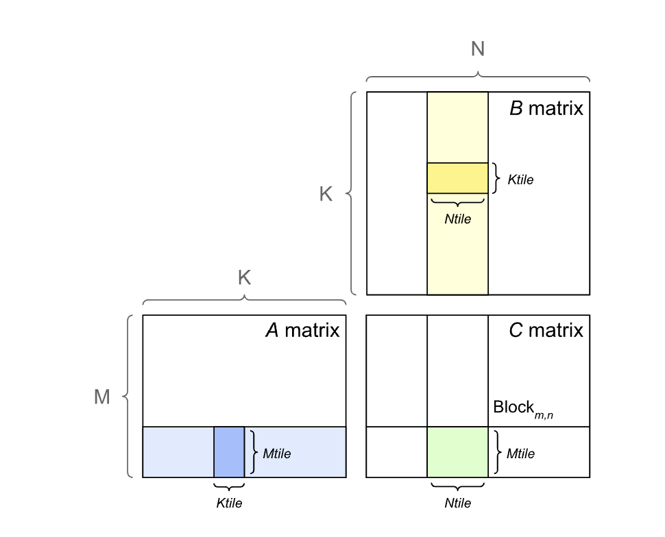
As we’ve observed previously, General Matrix Multiplications (GEMMs) is the most frequent operation in neural network layers. For the sake of the discussion, based on the conventions, let \(A \in \mathbb R^{m \times k}, B \in \mathbb R^{k \times n}\) and \(C = A \times \in \mathbb R^{m \times n}\). \(C\) would require a total of \(M*N*K\) fused multiply-adds (FMAs) (twice for the FLOPs). In general, for smaller multiplications, the operation is memory limited, and otherwise it is math-limited. As a consequence, vector products \(M = 1\) or \(N = 1\) are always memory limited and their arithmetic intensity is less than 1.
Implementation
Most of the GPUs implement matrix multiplication as a tiling operation - each thread block computes its output tile by stepping through the \(K\) dimension in tiles.
The latest NVIDIA GPUs have Tensor Cores to maximize multiplications in tensors. The performance is better when \(M, n< k\) are aligned to multiples of 16 bytes.
To aid with the code design, NVIDIA has provided the cuBLAS library that contains its optimized GEMM implementations. The tradeoff arises between parallelism and memory reuse - Larger tiles have fewer memory I/O but reduced parallelism. This is, in particular, a concern for smaller matrices. The library contains a variety of tiling to techniques to best utilize the GPU.
Dimension Quantization effects
A GPU function is executed by launching a number of thread blocks, each with the same number of threads. This introduces two potential effects on execution efficiency - tile and wave quantization.
- Tile Quantization - Tile quantization occurs when matrix dimensions are not divisible by the thread block tile size.
- Wave quantization - The total number of tiles is quantized to the number of multiprocessors on the GPU.
MI300X vs H100 vs H200
Source: MI300X vs H100 vs H200 Benchmark Part 1: Training; CUDA Moat Still Alive; SemiAnalysis
A case-study to examine why numbers on paper do not translate to real-life performance.

Comparing numbers on sheets is similar to comparing the megapixel count of cameras - the software is very important. NVIDIAs real world performance is also quite low compared to the papers. The analysis boils down to this - The potential on paper of AMD’s MI300X is not realized due to lack of AMDs software stack and testing. The gap between AMDs and NVIDIAs software is large - AMD is still catching up while NVIDIA is racing ahead. AMDs PyTorch is unfortunately broken.
Matrix Multiplication
OpenAI provides a do_bench function to benchmark matrix multiplications - it provides cache clearing between runs, ways to warmup and execute the benchmark multiple times and takes the median result. The results are as follows -

Notice how the marketed value is much higher than the real-world performance! The main finding from this study is that AMDs software stack is riddled with bugs that lowered its performance quite a lot.
It is also important to ensure that the underlying benchmark has no issues. For example, a popular benchmark for GEMM showed comparable performance for AMD and NVIDIA. However, on closer look, it had issues - it did not clear out L2 Cache and displayed the max performance rather than mean/median.
HBM Memory Bandwidth Performance
Higher HBM bandwidth leads to better inference performance. It is also helpful during training, specially with higher batch sizes.

Training Large Language Models
MLPerf GPT3 175B training is a good metric to measure the time it takes to train a model. However, this benchmark turned out to be very difficult for the AMD GPUs. Instead, the authors designed a benchmark better representing a user workload. They noted that many AI practitioners do not use Megatron, NeMo and 3D parallelism (advances in modern networks architectures for faster inference) due to their rigidity and complexity.
Overall for this test, on a single node, the authors obtained the following results -

The public releases of NVIDIA perform much higher than AMDs bugs-resolved builds. Apart from these single node builds, these providers also have a server cluster availability. NVIDIAs GPUs are merged with the NVLink fabric whereas AMD has xGMI. They connect up to 8GPUs with up to 450GB/s of bandwidth per GPU. This network of GPUs synchronize via the map-reduce command, and NVIDIAs topology performs better than that of AMDs.
Ironically, AMDs RCCI team has only 32 GPUs to experiment with the algorithms. Looking at this dismal conditions, TensorWave and SemiAnalysis sponsored some clusters to the team to aid the team in fixing their software.
Conclusion
Due to poor internal testing and a lack of good testing suite internally at AMD, MI300 is not usable out of the box. There have been advanced in attention mechanisms such as the FlexAttention that can improve the speed of window attention by 10-20x. However, due to the lacking nature of AMDs software, they are 6 months behind NVIDIA which is a long time in the rapid AI age.
In fact, many of AMDs libraries are forked off NVIDIA’s open-source libraries! The authors suggest AMD should hire more software talent to reduce the gap and reshape their user interface.
TVM: End-to-end compiler for Deep Learning
Current ML frameworks require significant manual effort to deploy on different hardware. TVM exposes the graph-level and operator-level optimizations to provide performance portability. In the current frameworks, techniques such as computational graph representations, auto-differentiation and dynamic memory management have been well established. Optimizing these structures on different hardware is however often infeasible, and developers have resorted to highly engineered and vendor-specific operator libraries. These libraries require significant amount of manual tuning and cannot be ported across devices.
How does the hardware matter? The input to hardware instructions are multi-dimensional, with fixed or variable lengths; they dictate different data layout and they have special requirements for memory hierarchy. These different constraints (memory access, threading pattern, hardware primitives - loop tiles and ordering, caching, unrolling) form a large search space that needs to be optimized to get efficient implementation.
TVM, an end-to-end ML compiler, has been designed to take a high-level specification of a deep-learning program from existing frameworks and generate a low-level optimized code for a diverse set of hardware backends. To do so, they made the following contributions
-
A tensor expression language to build operators and provide program transformation primitives to generate equivalent programs
-
An automated program optimization framework to find optimized tensor operators based on an ML cost model that adapts and improves based on the data received from the hardware backend.
-
A graph-rewriter compiler together the high-level and operator-level optimizations.
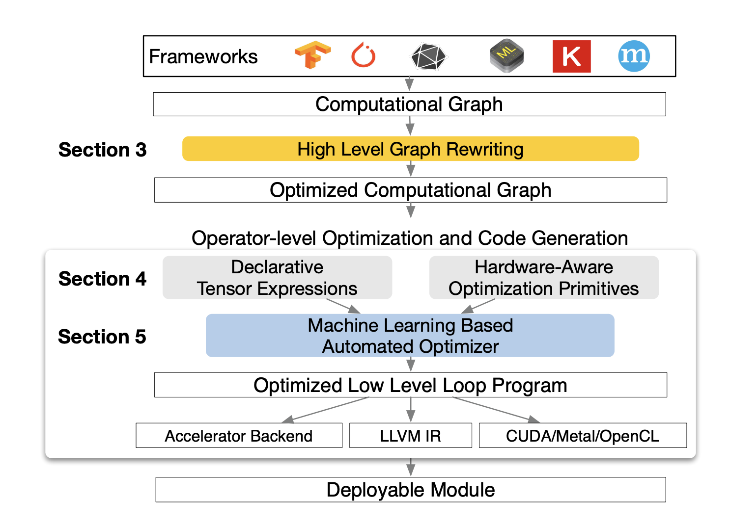
Graph Optimization
As mentioned previously, DL frameworks represent the data flow with graphs. This is different from the low-level compiler intermediate representation due to the presence of large, multi-dimensional tensors. Similar to compiler graph optimization, TVM also performs similar optimizations on this graph -
-
Operator Fusion - Fuse multiple small operations together, reducing the activation energy for executing each operator. The commonly used operators can be classified as injective (one-to-one, e.g., add), reduction (many-to-one, e.g., sum), complex-out-fusable (element-wise map based output, e.g., convolution), and opaque (cannot be fused, e.g., sort).
These classifications help us identify operators that can be combined. For example, in general
-
Multiple injective operators can be fused into one another
-
A reduction operator can be fused with the input injective operators
-
Complex-out-fusable operators can fuse element-wise operators to its output
These fusions generate up to 1.2x to 2x speedup!
-
-
Constant folding - Pre-compute graph parts that can be determined statically, saving execution costs
-
Static memory planning pass - Pre-allocate memory to hold each intermediate tensor
-
Data Layout transformations - Transform internal data layouts into back-end friendly forms. For example, a DL accelerator might exploit \(4\times4\) matrix operations, requiring data to be tiled into \(4\times4\) chunks. The memory hierarchy constraints are also taken into consideration.
These optimizations is where the search-space complexity arises. With more operators being introduced on a regular basis, the number of possible fuses can grow significantly considering the increasing number of various hardware back-ends as well. Doing these optimizations manually is infeasible and we need to automate the process.
Tensor Operations
TVM produces efficient code for each operator by generating many valid implementations for each hardware back-end and choosing an optimized implementation. This process is built on Halide’s idea of decoupling descriptions from computation rules and extends it to support new optimizations (nested parallelism, tensorization and latency hiding).
Tensor Expression and Schedule Space
Unlike high-level computation graph representations, where the implementation of tensor operations is opaque, each operation is described in an index formula expression language. For example, matrix multiplication is written as
m, n, h = t.var('m'), t.var('n'), t.var('h')
A = t.placeholder((m, h), name='A')
B = t.placeholder((n, h), name='B')
k = t.reduce_axis((0, h), name='k')
C = t.compute((m, n), lambda y, x:
                t.sum(A[k, y] * B[k, x], axis=k))
Each compute operation specifies both shape and expression for output. Since the language does not specify the loop structure and other execution details, it provides the flexibility for adding hardware-aware optimizations. Schedules are built incrementally with basic transformations to preserve the program’s logical equivalence. To achieve high performance on many back-ends, the schedule primitives must be diverse enough to cover various hardware backends.
Nested Parallelism
A common paradigm based on fork-join concept, nested parallelism is present in many existing solutions. Based on memory hierarchies, solutions also consider shared memory spaces and fetching data cooperatively. TVM builds on this idea with the concept of memory scopes to the schedule space so that a compute stage can be marked as shared. These shared tasks have memory synchronization barriers to ensure proper read/writes.
Tensorization
To ensure high arithmetic intensity, hardware developers have started implementing tensor compute primitives that consider the common operations and design specific hardware for their execution. They can improve the performance (similar to vectorization for SIMD architectures), but with more and more accelerators with their own variants of tensor instructions, there is a need for an extensible solution that can seamlessly integrate with all these.
To do so, TVM extends the tensor expression language to include hardware intrinsics. Doing so decouples the schedule from specific hardware primitives. The generated schedules are broken into a sequence of micro-kernel calls which can also use the tensorize primitive to make use of accelerators.
Explicit Memory Latency Hiding
Latency hiding refers to the process of overlapping memory operations with computation to maximize utilization of memory and compute resources. These strategies depend on the underlying hardware -
-
On CPUs, memory latency hiding is achieved implicitly with simultaneous multithreading or hardware prefetching.
-
GPUs rely on rapid context switching of many warps of threads
-
Specialized DL accelerators such as the TPU usually favor leaner control with a decoupled access-execute (DAE) architecture and offload the problem of fine-grained synchronization to software. This is difficult to program because it requires explicit low-level synchronization. To solve this, TVM introduces a virtual threading scheduling primitive that lets programmers specify a high-level data parallel program. TVM automatically lowers the program to a single instruction stream with low-level explicit synchronization.
Empirically, they observed that peak utilization increased by 25% for ResNet with latency hiding.
Automating Optimization
Now that we have a set of schedule primitives, TVM needs to find the optimal operator implementations for each layer of the DL model. An automated schedule optimizer automates optimizing the hardware parameters through a high-dimensional search space. It consists of
-
A schedule explorer that proposes new configurations. A schedule template specification API is used to let a developer define the changeable parameters in a code for a given hardware. TVM also has a generic master template to automatically extract possible knobs based on the tensor expression language. More the number of configurations, better optimization is possible.
-
A machine learning cost model that predicts the performance of a given configuration. Defining a perfect cost model is difficult - we need to consider memory access patterns, data reuse, pipeline dependencies, threading patterns, etc for every hardware. So, TVM uses a statistical approach by training an ML model that keeps getting better with newer data. The model has been chosen for quality and speed. The model uses a rank objective to predict the relative order of runtime costs. The model itself is a gradient tree boosting model (based on XGBoost) that makes predictions based on features extracted from the loop program.
The explorer starts with random configurations, and, at each step, randomly walks to a nearby configuration. This exploration method is more efficient than random exploration.
A distributed device pool scales up the running of on-hardware trials and enables fine-grained resource sharing among multiple optimization jobs.
Summary
The core of TVM is implemented in C++ with approximately 50k lines of code. It achieves significantly higher performance as compared to earlier works. However, even with this extensive approach, the models can be designed carefully to achieve much better performance. For example, as seen in Flash Attention, the optimization is a result of human intellectual effort rather than a manual exploration of a partially defined search space by an automated compiler.
Triton: An intermediate language and compiler for Neural Network computations
As with the previous motivation, Triton was developed to provide a way for users to test new models efficiently without needing to manually optimize it for the hardware. Triton is a language and a compiler centered around the concept of tile, statically shaped multi-dimensional sub-arrays. It is a C-based language for expressing tensor programs in terms of operations on parametric tile variables and provides novel tile-level optimization passes for compiling programs into efficient GPU code.
Previous approaches to tackle the wide-variety of deep-learning models include Domain-Specific Languages (DSLs) based on polyhedral machinery (tenor comprehensions) and/or loop synthesis techniques (Halide, TVM, PlaidML, etc). These systems perform well for models such as depthwise-separable convolutions, but they are much slower than vendor-based libraries like cuBLAS and cuDNN. The problem with vendor based libraries is that they support only a restricted set of tensor operations.
These issues have been addressed by the use of micro-kernels - hand-written tile-level intrinsics, but it requires significant manual labour and cannot be generalized. Compilers do not support these tile-level operators and optimizations. The prior approaches can be summarized as
-
Tensor level IRs - XLA, Flow to transform tensor programs into predefined LLVM-IR and CUDA-C operation templates (e.g., tensor contractions, element-wise operations, etc) using pattern matching. Triton provides more flexibility.
-
The polyhedral model - Tensor Comprehensions (TC), Diesel to parameterize and automate the compilation of one of many DNN layers into LLVM-IR and CUDA-C programs. Triton supports non-affine tensor indices.
-
Loop synthesizers - Halide, TVM to transform tensor computations into loop nests that can be manually optimized using user-defined schedules. Automatic inference of possible execution schedule in Triton.
Triton-C
A C-like language for expressing tensor programs in terms of parametric tile variables. It provides a stable interface for existing DNN trans-compilers and programmers familiar with CUDA. Here is an example of matrix multiplication
// Tile shapes are parametric and can be optimized
// by compilation backends
const tunable int TM = {16, 32, 64, 128};
const tunable int TN = {16, 32, 64, 128};
const tunable int TK = {8, 16};

// C = A * B.T
kernel void matmul_nt(float* a, float* b, float* c, int M, int N, int K) {
    // 1D tile of indices
    int rm[TM] = get_global_range(0);
    int rn[TN] = get_global_range(1);
    int rk[TK] = 0...TK;

    // 2D tile of accumulators
    float C[TM, TN] = {0};

    // 2D tile of pointers
    float* pa[TM, TK] = a + rm[:, newaxis] + rk * M;
    float* pb[TN, TK] = b + rn[:, newaxis] + rk * K;

    for (int k = K; k >= 0; k -= TK) {
        bool check_k[TK] = rk < k;
        bool check_a[TM, TK] = (rm < M)[:, newaxis] && check_k;
        bool check_b[TN, TK] = (rn < N)[:, newaxis] && check_k;

        // Load tile operands
        float A[TM, TK] = check_a ? *pa : 0;
        float B[TN, TK] = check_b ? *pb : 0;

        // Accumulate
        C += dot(A, trans(B));

        // Update pointers
        pa = pa + TK * M;
        pb = pb + TK * N;
    }

    // Write-back accumulators
    float* pc[TM, TN] = c + rm[:, newaxis] + rn * M;
    bool check_c[TM, TN] = (rm < M)[:, newaxis] && (rn < N);
    @check_c * pc = C;
}
It is a front-end to describe CUDA like syntax with Numpy like semantics. The syntax is based on ANSI C, and has the following changes
-
Tile declarations: Syntax for multi-dimensional arrays that can be made parametric with
tunablekeyword. Ranges with ellipses. -
Broadcasting using
newaxiskeyword -
Predicated statements in tiles with
@
A tile is an abstraction to hide details involving intra-tile memory coalescing, cache management and specialized hardware utilization.
The triton programming model is similar to that of CUDA - each kernel corresponds to a single thread execution.
Triton-IR
An LLVM-based Intermediate Representation (IR) that provides an environment suitable for tile-level program analysis, transformation and optimization. Triton-IR programs are constructed directly from Triton-C during parsing, but automatic generation from embedded DSLs is unimplemented. Here is an example for the max operation
define kernel void @relu ( float * %A , i32 %M , i32 % N ) {
prologue :
% rm = call i32 <8 > get_global_range (0) ;
% rn = call i32 <8 > get_global_range (1) ;
; broadcast shapes
%1 = reshape i32 <8 , 8 > % M;
% M0 = broadcast i32 <8 , 8 > %1;
%2 = reshape i32 <8 , 8 > % N;
% N0 = broadcast i32 <8 , 8 > %2;
; broadcast global ranges
%3 = reshape i32 <8 , 1 > % rm;
% rm_bc = broadcast i32 <8 , 8 > %3;
%4 = reshape i32 <1 , 8 > % rn;
% rn_bc = broadcast i32 <8 , 8 > %4;
; compute mask
% pm = icmp slt % rm_bc , % M0;
% pn = icmp slt % rn_bc , % N0;
% msk = and % pm , % pn;
; compute pointer
% A0 = splat float * <8 , 8 > % A;
%5 = getelementptr % A0 , % rm_bc ;
%6 = mul % rn_bc , % M0;
% pa = getelementptr %5 , %6;
; compute result
% a = load % pa;
% _0 = splat float <8 , 8 > 0;
% result = max % float %a , % _0;
; write back
store fp32 <8 , 8 > % pa , % result
}
It is similar to LLVM-IR, but it includes the necessary extensions for tile-level data-flow and control-flow.
It constructs a data-flow graph including nodes for multi-dimensional tiles and instructions made from basic blocks of code. The control-flow is handled with the use of Predicated SSA and \(\psi\)-functions (compare and merge).
Triton-JIT compiler
A Just-In-Time (JIT) compiler and code generation backend for compiling Triton-IR programs into efficient LLVM bitcode. It includes
-
A set of tile-level, machine-independent passes aimed at simplifying input compute kernels independently of any compilation target. It involves operations such as pre-fetching to reduce cache misses and tile-level peephole optimization that implement algebraic tricks with tensors.
-
A set of tile-level, machine dependent passes for generating efficient GPU-ready LLVM-IR. It involves
-
Hierarchical Tiling - The tiles defined by the user are further broken down to the machine’s constraints.
-
Memory coalescing - Making sure that adjacent threads simultaneously access nearby memory locations.
-
Shared memory allocation - To improve memory reuse.
-
Shared memory synchronization - Barriers to preserve program correctness in parallel execution.
-
-
An auto-tuner that optimizes any meta-parameters associated with the above passes. Traditional auto-tuners rely on hand-written templates. In contrast, Triton-JIT extracts optimization spaces from Triton-IR (hierarchical tiling parameters only - up to 3 per dimension per tile) and optimizes using an exhaustive search. This needs to be improved in the future
Summary
Triton defeats the other prior solutions achieving performance close to DSLs. However, the authors have highlighted many areas where this framework can be improved in the future - support for tensor cores (the ones TVM talked about), implementation of quantized kernels and integration into higher-level DSLs.
Deep Compression: Compressing Deep Neural Networks with Pruning, Trained Quantization and Huffman Coding
Released in 2016, Deep Compression is a three stage-pipeline involving pruning, trained quantization and Huffman coding that reduce the storage of neural networks by \(35\times\) to \(49\times\) without affecting their accuracy! Here are these steps in detail
-
Network Pruning- Leveraging the previous successes of pruning CNNs, the authors prune the network by removing all connections with weights below a certain threshold from the network. The model is retrained to learn optimized weights. This step reduces the number of parameters by almost \(10\times\) for AlexNet and \(35\times\) for VGG-16.
For further storage savings, these weights are stored as a compressed sparse row/column. Moreover, the authors recommend storing the index different instead of absolute position, and they assign the bits very parsimoniously.
-
Trained Quantization and Weight Sharing - A quantization technique during training, that essentially shares the weights across multiple neurons. That is, the updates and computes are grouped as centroids. The compression rate with this technique is given by
\[r = \frac{nb}{n \log_2(k) + kb}\]where \(k\) is the number of clusters, \(n\) is the number of connections in the network, and \(b\) is the number of bits used to encode these connections. The weights are not shared across layers, and the quantization is done so that the loss across all the weights is minimum. The weights centroids can be accessed through a hash function.
The authors go into some more detail about initializing these centroids.
-
Forgy (Random) - Randomly chooses \(k\) observations from the dataset. These centroids tend to concentrate near the peaks of the weight distribution.
-
Density based initialization - Starts with a uniform distribution of the centroids and then adapts to the PDF of the data distribution. The centroids still gather near the peaks but have a better spread than random initialization.
-
Linear initialization - Most scattered initialization
Why do these matter? In many cases, the larger weights are important but they usually are fewer in number. So, the first two initializations that are centered around the distribution peaks (which are not the large values) can result in poor accuracy. So, linear initialization usually works the best. They also experimentally confirm these hypotheses.
-
-
Huffman Coding - Huffman encoding is the optimal encoding standard that relies on a common prefix code for lossless data compression. The intuition is that more common symbols are represented with fewer bits. The authors of this paper use this idea to encode the sparse matrix formed by the quantized weights. The distributions are usually bi-modal and Huffman encoding saves 20-30% in storage with these non-uniform distributions.
Overall, with all these methods combined, the pipeline saves over \(30\times\) in storage for many image models! What’s more? The accuracy is more or less the same as the original models!
The authors analyze a bit more on how these methods work together with one another. They noticed that the accuracy of the networks starts dropping sharply after a certain threshold in each method.
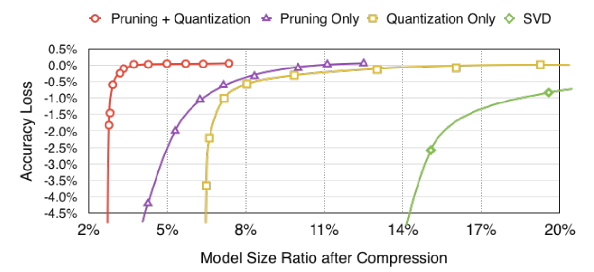
They also point out that quantization works well with pruned networks due to lesser number of parameters to quantize. In fact, they notice that pruning virtually does not affect the performance obtained after quantization. Basically, with more savings, you get the same performance.
The target of this paper is to allow models to work on edge devices. They perform experiments on latency, especially with the fully connected layers since they occupy 90% of the parameters in the networks. One must note that benchmarking quantized models is difficult since there are no hardware primitives to support the lookup architecture for centroid codes. They have the following observations
-
Matrix vector multiplications are more memory-bound than matrix matrix multiplications, and so reducing the memory-footprint for non-batched inferences is important.
-
Pruned networks had \(3\times\) speed-up since larger matrices are able to fit into the caches.
-
They also note that the effect of the quantization codebook is negligible as compared to the other operations.
In the future, they emphasize that to take full-advantage of the method, hardware must support indirect matrix entry lookup and the relative indices in CSC and CSR formats. This can be achieved via custom software kernels or hardware primitives.
A survey of Quantization methods for Efficient Neural Network Inference
The research and development of efficient ML has been a constant interest alongside developing new ML architectures. The earlier works in this space include:
-
Optimizing the micro-architecture (such as depth-wise convolution, low-rank factorization) and macro-architecture (residual connections, inception). These methods have been a result of manual search that is not scalable. A new line of work called AutoML and Neural Architectural Search methods was developed to automate the search of the right ML architecture under the given constraints of model size. Another line of work in ML compilers tried to optimize a particular architecture for a specific hardware.
-
Pruning the models by removing the neurons with small saliency (sensitivity - that do not affect the result of the network largely). These methods can be categorized as
-
Unstructured - Removes neurons with smaller saliency wherever they occur - this tends to be aggressive while having little impact to performance. However, this approach leads to sparse matrix operations that are harder to accelerate and are memory bound.
-
Structured - A group of parameters (e.g., entire convolutional filter) is removed so that the operations are still on dense matrices.
-
-
Knowledge distillation refers to training large models and using it as a teacher to train a compact model. The idea is to use the soft-probabilities generated by the teacher to better train a small model, resulting in high compression. This class of methods can significantly reduce the model size with little to no performance degradation.
-
Quantization has showed consistent success for both training and inference of Neural Networks. It allowed breakthroughs such as half-precision and mixed prevision training to have a high throughput in AI accelerators.
Quantization is loosely related to some works in neuroscience which suggest that information stored in continuous form will inevitably get corrupted by noise. However, discrete signal representations can be more robust.
Quantization is mainly useful for deploying models on edge devices. Quantization, combined with efficient low-precision logic and dedicated deep learning processors can really push edge processors.
History of Quantization
Quantization maps input values in a large (often continuous) set to output values in a small (often finite) set. The effect of quantization and its use in coding theory was formalized with the seminal paper by Shannon in 1948. It evolved into different concepts such as Pulse Code Modulation in signal processing.
In digital systems, numerical optimization methods showed that having quantization effects produces roundoff errors in applications that we know to have closed form solutions. These realizations led to a shift towards approximation algorithms.
Neural Network (NN) quantization is different from these earlier considerations. Since inference and training of NNs is expensive and NNs are typically over-parameterized, there is a huge opportunity to reduce the precision without impacting accuracy. The nature of NNs allows high error/distance between quantized and non-quantized models. Also, the layered nature of NNs allows exploration of more types of quantizing techniques.
There are two kinds of quantization
-
Uniform quantization - \(Q(r) = Int(r/S) - Z\) where \(Q\) is the quantization operator, \(r\) is a real valued input (activations and weights), \(S\) is a real-valued scaling factor and \(Z\) is an integer zero-point. The resulting quantized values are uniformly spaced. An important factor is the choice of the scaling factor \(S\). It is determined by the clipping range that can be determined from calibration. Based on the clipping range, symmetric quantization results in easier implementation since it results in \(Z = 0\). These calibration ranges can be computed dynamically for every activation map or done statically during inference.
-
Non-uniform quantization - Essentially, the quantized values are not necessarily uniformly spaced. It typically achieves higher accuracy for cases involving non-uniform distributions. Neural networks usually have bell-shaped distributions with long tails. These methods can be generally considered as optimizing the difference between the original tensor and quantized counterpart. The quantizer itself can also be jointly trained with the model parameters.
These prior approaches can be classified as rule-based and optimization-based quantizations. In addition, there can be clustering based quantizations such as K-means to minimize the performance loss.
The granularity of quantization is also an important choice -
-
Layerwise quantization - The clipping range is determined by considering all the weights in convolutional filters of a layer.
-
Groupwise quantization - The clipping range is determined by grouping multiple channels inside a layer to account for cases where the distribution of the parameters across a single convolution/activation varies a lot.
-
Channelwise quantization - Each channel is assigned a dedicated scaling factor.
-
Sub-channelwise quantization - Each channel is partitioned into groups that have their own scaling factor.
These quantization methods can also be applied during training and after training
-
Quantization-aware training (QAT) - The NN is re-trained with quantized parameters to improve the accuracy that degrades due to the perturbations caused by quantization. In one such method, the forward and backward passes are performed on the quantized model in floating point and then quantized after each gradient update. The back-propagation through a quantization operator is approximated via Straight-Through Estimator (STE) that ignores the rounding operation and approximates with an identity operation. It often works well in practice except for binary quantization. Other approaches include combinatorial optimization, target propagation or Gumbel-softmax. There has been a lot of work with regards to this aspect of quantization.
The other kind of approaches tried learning quantization parameters during the training. These are recent works and there is not much to summarize here. In summary QAT methods require retraining efforts which may not be worth it for short-lived models.
-
Post-training quantization (PTQ) - In contrast to QAT, the overhead is very low, does not require retraining, and it can be applied in situations where data is limited or unlabeled. However, it comes at a cost of lower accuracy. To prevent this, many approaches were proposed - bias correction methods for post-quantization ranges, analytically optimizing the clipping ranges, L2 distance optimization, outlier channel splitting, adaptive rounding methods, etc.
-
Zero-shot quantization - In cases where the original data is not available to find the clipping range, zero shot quantization is used. It can again be classified into two levels based on if the approach has fine-tuning after quantization. Some approaches try to generate synthetic data to mimic the real data (earlier approaches included GANs for this) and calibrate the clipping ranges. In summary, these methods are useful for Machine Learning as a Service providers where security and privacy are a concern.
Finally, there is a notion of stochastic quantization wherein the floating numbers are mapped up or down with a probability associated to the magnitude of the weight update. Phew, that finishes the background.
Quantization below 8 bits
-
Simulated and Integer-only Quantization - Simulated quantization refers to storing parameters as lower precision but carrying out calculations as floating point. This method can lead to higher stability while training and better inference performance, but results in mixed representation calculations. It is useful for problems that are bandwidth-bound rather than compute-bound such as in recommendation systems. The latter method which uses only a single format can exploit some hardware optimizations and be more energy efficient.
-
Mixed-Precision Quantization - In this method, each layer is quantized with different bit precision to improve the accuracy. Searching the mixed-precisions for the layers is essentially a search problem. Researchers have tried RL abased exploration methods or using a neural network to achieve this, but these can be computationally intensive with their performance being sensitive to hyperparameters and initialization.
Another class of mixed-precision methods uses periodic function regularization by automatically distinguishing different layers and their importance wrt accuracy to learn their bandwidths. Some approaches also proposed a linear programming formulation for this approach. With hardware supporting these types of methods, it can be a feasible option for many cases.
-
Hardware Aware Quantization - Essentially considering hardware factors such as on-chip memory, bandwidth and cache hierarchy to choose the quantization parameters. Again, it is a search problem.
-
Distillation-Assisted Quantization - Some approaches tried to use model distillation to boost quantization accuracy. This method has to be studied separately since it was not covered in the survey.
-
Extreme Quantization - Binarization. Many researchers have been bold enough to try this. Important works include
-
Binary Connect - Weights are +1 or - 1
-
Binarized NN - Binarizes both activations and weights. Has improved latency due to matrix multiplications being replaced by XNORs and bit-counting.
-
XNOR-Net - Same as before but the weights have a scaling factor. Further works noted that weights tend to be close to 0, and adopted a ternarization (yes, that’s a word).
Nevertheless, these result in significant performance degradation. The works in this field can be classified as Quantization error minimization, Improved loss function formulations, and improved training methods. People tried to do this with BERT and GPT models as well!
-
-
Vector Quantization - Borrowing ideas from signal processing, these approaches include clustering weights or methods such as product quantization that subgroups the vectors.
Future Directions, Summary and Conclusion
-
Quantization should be provided as a plug-and-play module in software packages to improve the accessibility.
-
Hardware and Neural networks should be co-designed to optimize the computations.
-
As mentioned in the previous article, coupling compression methods can have a huge impact!
Distributed Training and Efficient Finetuning
The growth of machine learning is much faster than what hardware can catch up with. We cannot fit our models in a single GPU anymore, and we need to learn how to use distributed training systems to satisfy our training needs.
Typically, we deal with large model sizes (10B+) and large dataset sizes (1T+ tokens while pre-training, 1M+ in supervised fine-tuning). The goal is to maximize throughput by using smart distributed training strategies, where each GPU worker only deals with the fraction od training state and date. The main strategies used for this are -
-
Data Parallelism (DP) - Each GPU worker gets a fraction of the total mini-batch of data, and computes the gradients on that data. these are then averaged across the workers to update the weights. In the most basic form, each worker has a copy of model weights, optimizer state and gradients for the fraction of the data it’s working on
-
Model Parallelism (MP, Vertical) - Models are vertically sliced with different layers placed on different GPUs. In the naïve form, the GPUs wait for the previous GPU to finish the computation. To improve this, people use pipeline parallelism where the execution is pipelined across micro-batches.
-
Tensor Parallelism (TP) - Each GPU processes only a slice of a tensor by horizontally slicing the model across GPU workers. Each worker process the same batch of data but for different activations. They exchange parts when needed.
These are the core strategies but there can be hybrid approaches based on the needs.
ZeRO-powered Data Parallelism
DeepSpeed’s ZeRO (Zero-Redundancy) is one of the most efficient and popular strategies for distributed training. It is a data parallelization strategy that leverages memory redundancy in data-parallel training and the inter-GPU connects to improve throughput. It comprises of two components - ZeRO-DP (data parallelism) and ZeRO-R (residual memory). The team has also proposed newer architectures such as ZeRO-Offload/Infinity (offloading computation to CPU/ NVMe disk) and ZeRO++ (with flexible multi-node training and quantized weights).
It boasts up to 64x memory reduction for a specific example across different hardware setups and model sizes!
The base method is PyTorch DDP that has been described before. Each GPU worker has a copy of the model weights, optimizer state and gradients. To average the gradients, all-reduce step is used. All-reduce is a two-step approach - reduce-scatter operation to reduce different parts of the data on different processes and an all-gather operation to gather the reduced data on all the processes. It requires \(2\psi\) amount of communication cost for \(\psi\) number of parameters. The paper suggests three ways of doing this -
-
ZeRO Stage 1 / \(P_{os}\) (Optimizer state partitioning) - The optimizer state is partitioned/sharded across the workers, with model weights and gradients replicated across all the workers. Previously, the all-reduce step gets the average gradient value across all the workers. Now, each worker updates the optimizer state with the Adam equations that is in it’s partition. The key savings come from using a sharded optimizer state rather than having copies. Recall that Adam optimizer uses 2x as many weight parameters as the model.
-
ZeRO Stage 2 / \(P_{os + g}\) (Optimizer State + Gradient Partitioning) - As the name suggests the gradients are sharded along with the optimizer state. So each worker calculates its gradient and the gradients are averaged with reduce-scatter at the worker (instead of all-reduce).
-
ZeRO Stage 3 / \(P_{os + g}\) (Optimizer State + Gradient Partitioning) - The partitioning of the model weights is done horizontally. That is, each layer of the model is split across the GPUs and there is a parameter communication on-demand. The communication volume increases (since there is an extra all-gather for model parameters, the communication becomes 3x the number of parameters). As a consequence, the memory consumption is cut down by the number of GPU workers \(N\) which is huge! So if you have enough number of GPUs, you can get good savings on the memory.
These were the base methods. The authors proposed a wide-array of variations on top of this.
-
ZeRO-R - Improves on ZeRO-DP by reducing the memory consumptions by activations and managing memory fragmentation. It essentially shards the activations as well. it also uses some temporary buffers to store intermediate results during gradient accumulation and reduction across workers.
-
Zero-Offload - The idea is to offload optimizer and computation from GPUs to the host CPU. Back in 2021, this obtained magnitudes of higher performance over PyTorch DDP. CPU computation is much slower, so only the less-intensive operations are offloaded so that the total compute complexity stays the same. So, operations such as norm calculations, weight updates, etc are done on the CPU, while the forward and backward pass are done on the GPU. It works with all stages of ZeRO (1, 2 and 3).
-
Zero-Infinity - An improvement on the previous approach to allow offloading to disk and some more improvements to CPU offloading. It could fit 10-100T parameters on just one DGX-2 node! This method is specifically built on top of ZeRO-3, and they achieved 49 Tflops/GPU for a 20 trillion model spread across 512 GPUs. This is insane!
-
ZeRO++ - The latest improvement in this saga of approaches. The major changes are quantized weights (reduces communication by half), hierarchical partitioning (a hybrid sharing technique) and quantized gradients.
Fully-Sharded Data Parallel
FSDP is another data-parallelism technique aimed at improving memory efficiency with limited communication overhead. It’s based on the previous approaches and has two sharding strategies - Full Sharding and Hybrid Sharding.
- Full-sharding - Similar to ZeRO-3, the parameters, optimizer state and gradient are sharded across workers.
The high level procedure is -
In forward path
- Run all_gather to collect all shards from all ranks to recover the full parameter in this FSDP unit
- Run forward computation
- Discard parameter shards it has just collected
In backward path
- Run all_gather to collect all shards from all ranks to recover the full parameter in this FSDP unit
- Run backward computation
- Run reduce_scatter to sync gradients
- Discard parameters
- Hybrid Sharding - It consists of both sharding and replication based on the tradeoff between communication latency and memory savings. This option is useful when the only way out is sharding parameters.
Implementation in Practice
ZeRO and FSDP integrate well with existing architectures. ZeRO is implemented in Microsoft’s DeepSpeed library and is integrated into the 🤗 Accelerate library. FSDP is a part of PyTorch itself, and again has an integration in the 🤗 Accelerate library.
Pipeline parallelism requires architectural changes in the forward pass of the model. For this, the best option right now is Megatron-LM that is discussed next. A recent update in 2024 pushed nanotron that has 3D parallelism support.
Efficient Fine-tuning
Some popular optimizations -
-
Mixed precision - It has been widely adopted form LLMs wherein there is a master copy that is updated from the gradients of quantized copies.
-
Parameter Efficient Fine Tuning (PEFT) - Various methods to reduce the finetuning effort.
-
Flash-attention - It is a fast, memory efficient, exact, IO-aware attention mechanism. FlashAttention 2 achieves 220+ TFLOPS on A100! FlashAttention 1 achieved 124 TFLOPs before. However, these only support Ampere, Ada and Hopper NVIDIA GPUs and half prevision data types.
-
Gradient and Activation Checkpointing - A technique wherein only a subset of intermediate activations are stored and others are recomputed when needed. However, it can slow down the training by 20% for \(O(\sqrt N)\) memory savings. Check this site for better info.
-
Quantization - Post-training quantization refers to savings at inference since weights don’t change. During training, there can be updates with quantized parameters. QLoRA is one such technique that quantizes the base model and trains half precision low-rank weights on this. The throughput actually decreases due to the de-quantization step for each activation. Nevertheless, it can reach the performance of full fine-tuning.
-
Gradient accumulation - The intuition behind this approach is to run the network in micro-batches, accumulate the gradients across these micro-batches and update the model for a full batch-size. The idea is to get the same output as with large batches but with much lower memory consumption (the time increases accordingly). Larger batches usually have lower convergence time and the technique is especially useful when using multiple GPUs. However, one should be conservative with this approach. A pre-transformers era paper showed larger batch sizes can reduces the generalization abilities of a model.
Summary
The final tips for training these large models from this article are -
BF16/ FP16 by default. BF16 comes with basically no other config parameters and usually without any overflow issues (as opposed to FP16, where you can get different results with different loss scaling factors and have more overflow issues because of smaller dynamic range), so it’s very convenient.
Use (Q)LoRA with trainable parameters added to all the linear layers.
Use Flash Attention if your GPU supports it. Currently, Flash Attention 2 is supported for Llama 2 and Falcon in HuggingFace, with other models requiring monkey patches.
Use Gradient/Activation Checkpointing. This will reduce throughput slightly. If you’ve got Flash attention, gradient checkpointing might not be required (they use a selective gradient checkpointing in the softmax of the attention layer).
Use an efficient sampler in your dataloader, like the multi-pack sampler.
If you have multiple GPUs, always try BF16 + LoRA + Gradient Checkpointing + DeepSpeed ZeRO 3 first. Megatron stuff from the next part too
Use quantization when you have very limited GPU memory. QLoRA-style training currently works for DeepSpeed ZeRO 1/2 only. Thus, even though it is memory efficient when it comes to model parameters, you still have parameter redundancy with ZeRO 1/2, and you also get reduced throughput.
With more and more GPUs (say 8 V100s or A100s), DS ZeRO-3 should be the way to go. DS ZeRO-2 is also good, but you can start to hit CPU RAM limits (during model initialization) because of model parameters being replicated across all workers.
In a small-scale multi-node setup, with a few nodes, the best option seems to be DeepSpeed ZeRO-3 with hierarching partitioning enabled (or FSDP with hybrid sharding). If you’ve got Infiniband interconnect, you can mostly use plain DeepSpeed ZeRO-3 and push for larger model sizes as well.
Gradient accumulation should be used if you’re still short on batch size after all the above optimizations. Training times with gradient accumulation can be faster with large models and multi-GPU/ multi-node settings.
If you’re really short on GPU memory, then you would activate CPU/ disk offloading (and by disk, this has to be NVMe for ZeRO-Infinity). With the advent of Flash Attention 2, we need another study on the throughput gap between plain GPU-based training and GPU + NVMe/CPU-offloading. ZeRO-Infinity is better than ZeRO-Offload.
Calculate the effective batch size and adjust hyperparameters accordingly. A general guideline is to scale up the learning rate with the effective batch size. This seems to hold true even for 100B+ models, as seen in OpenAI’s finetuning docs.
Finally, when you do start training, monitor
htopto check on RAM usage (sometimes RAM OOM can be an issue), along withnvidia-smito make sure GPUs aren’t bottlenecked by data preprocessing (you should aim for close to 100% volatile GPU utilization, even if GPU memory usage is lesser).Lower learning rate during pre-training works better in practice for GPT-3 and Bloom paper. The intuition/explanation for this effect is still pending.
Megatron-LM
A simple model parallel approach that is orthogonal and complementary to pipeline model parallelism. They also show that larger models do indeed result in higher performance by demonstrating larger models trained with their approach.
Their approach exploits the inherent structure of transformer based language models that trains efficiently with PyTorch. Compared to the baseline that trains a 1.2 billion parameter model on a single NVIDIA V100 32GB GPU that sustains 39 TFLOPs (30% of the peak possible value), their method obtains 15.1 PetaFLOPs with an 8.3 billion model on 512 GPUs with 8-way parallelism - 76% scaling efficiency.
The paper mentions the previous approaches gradient accummulation (Valiant, 1990) and gradient/activation checkpointing (Chen et. al., 2016), and that they are constrained to fit the model on a single GPU. They also mention that layer parallelism suffers from pipeline bubbles that reduce efficient or changes to the optimizer that impacts accuracy. Distributed tensor computation is a more general approach, and the authors use this technique for transformer’s attention heads to parallelize. No framework, no compiler, simple PyTorch modifications.
Model Parallel Transformers
The core idea is to parallelize the transformer architecture with some synchronization primitives.
-
The MLP part is a GEMM followed by a GeLU non-linearity.
\[\begin{align*} Y &= GeLU(XA) \\ &= GeLU (\begin{bmatrix} X_1 & X_2\end{bmatrix}\begin{bmatrix}A_1 \\A_2\end{bmatrix}) \\ & \neq GeLU(X_1A_1) + GeLU(X_2A_2) \end{align*}\]The matrix \(A\) can be split across rows and \(X\) across columns. Due to the non-linearity of \(GeLU\), this method would need a synchronization point before the non-linear layer.
The other approach is to split \(A\) across columns, and then \(GeLU\) can be applied independently. It doesn’t require any synchronization point.
\[\begin{align*} Y &= GeLU(XA) \\ &= GeLU (X \begin{bmatrix} A_1 & A_2\end{bmatrix}) \\ &= GeLU(XA_1) + GeLU(XA_2) \end{align*}\]This approach splits both GEMMs in the MLP block across GPUs and requires a single all-reduce operation in the forward and backward passes.
-
For the self-attention block, the partitioning of GEMMs is done in a similar column parallel fashion for \(K, Q, V\). These outputs can directly be passed into the linear layer to parallelize across rows evading communication latency here as well. The final answers after the FFN can be fused within two all-reduce operations.
Furthermore, since vocabulary sizes can be large, it is beneficial to parallelize the output embedding GEMM. However, since the output embedding layer shares weights with the input embedding, the input embedding matrix is also parallelized across the vocabulary dimension. These splits would add two all-reduce operations. However, in the output layer the all-gather operation can be optimized by fusing with the cross-entropy loss - reduces parameter communication from \(b\times s\times v\) to \(b \times s\). That is, communicating scalar losses instead of logits is a huge reduction in communication.
The paper further reduces the communication by replicating dropouts, layer normalization, and residual connections across GPUs and only the results are communicated.
Specifically, each worker maintains duplicate copies of layer normalization parameters on each GPU, and run dropout and residual connection on the output of the model parallel region before feeding them as input to the next model parallel regions. To optimize the model, each worker optimizes its own set of parameters. Since all values are either local to or duplicated on a GPU, there is no need for communicating updated parameter values in this formulation.
Conclusion
The authors provide comprehensive set of results to demonstrate their method with GPT-2 and BERT, showcasing that they are able to scale the compute much higher with these simple optimizations while achieving higher accuracy with larger models. They also found that BERT like models perform better with layer normalization.
GPipe
GPipe is an attempt to democratize model parallelism through pipeline algorithms for layered networks. It was proposed towards the end of 2018, when transformers started getting popular and the hardware could not catch up. The high-level idea is that each model can be specified as a sequence of layers and consecutive groups of layers can be partitioned into cells that are each placed on a separate accelerator. A novel pipeline parallelism algorithm with micro-batch splitting is used to maximize the utility of the hardware.
It was released to the public as an open-source library. The interface consists of user-selectable parameters such as estimate of the computation cost \(C_k\), number of partitions \(K\), number of micro-batches \(M\), and layers \(L\) that define the model etc.
GPipe is a synchronous pipeline based parallelism technique. There are other approaches that split the operators across the accelerators (GPipe splits the layers), akin to SIMD approach for data parallelism. They call this the Single Program Multiple Data (SPMD) paradigm, and Mesh-Tensorflow is one method existing at that time. They note that these methods have high communication overhead and there are variety of ways of splitting the operators some of which may not be generalizable or scalable. Along similar lines, PipeDream pipelines the execution of forward passes and intersperses them with backward passes to maximize hardware utilization. However, it suffers from update staleness introduced by asynchronous backward updates. Some versions suggested maintaining multiple versions of the model, but that greatly hampers the scaling abilities of the technique.
Algorithm
GPipe partitions the network into \(K\) sequential cells and each of them are placed on the available devices. Communication primitives are inserted at the boundaries to allow data transfer. The partitions are split so that the variance across all the cells is minimized to sync the computation time across all partitions.
During the forward pass, every mini-batch of size \(N\) is split into \(M\) micro-batches that are pipelined through \(K\) accelerators. During the backward pass, gradients for each micro-batch are computed with the weights used for the forward pass, and these gradients are accumulated to update the model parameters across all accelerators.
For batch-normalization layers, the statistics of inputs across micro-batches and moving averages across the mini-batch are calculated and communicated.
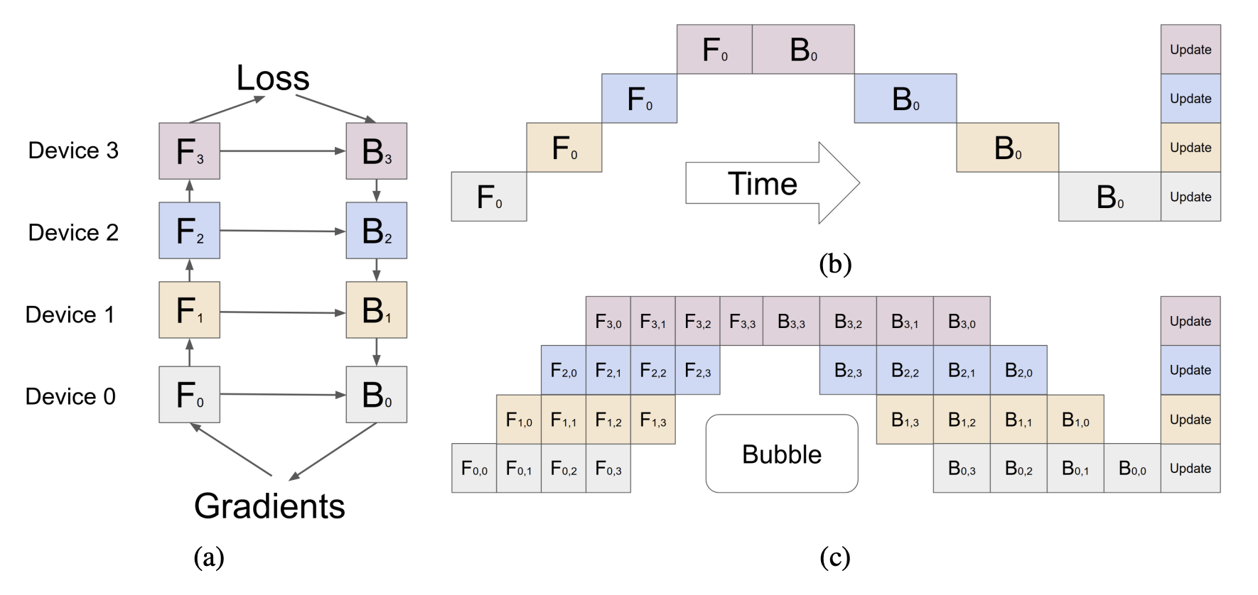
To further decrease the memory consumption, GPipe supports gradient checkpointing - each accelerator only stores the output activates at the partition boundaries. As a result, the peak activation memory is reduced to \(O(N + \frac{L N }{KM})\) from \(O(NL)\) (without gradient checkpointing and partitioning) where \(N/M\) is the micro-batch size and \(L/K\) is the number of layers per partition.
The bubble overhead with this method is \(O(\frac{K - 1}{M + K - 1})\) amortized over the number of micro-steps \(M\). It is negligible in practice when \(M \geq 4\times K\). Note that increasing the number of micro-batches would underutilize the GPUs.
GPipe has low communication overhead allowing efficient scaling on accelerators without high-speed interconnects. However, the memory requirements and computation flops at different layers are usually very imbalanced leading to inefficiencies. The authors left this problem of better partitioning algorithms to future works.
Results and Conclusion
GPipe is able to reduce the memory requirements by half allowing training of almost 25x larger models. These savings are even more significant with architectures such as transformers where the savings can be 250 times. The speed-up is almost linear barring the pipeline bubbles and communication overheads. They obtained significant savings even with a low-speed communication device (PCI-E vs NVLink).
These savings translate into the model performance as well. Giant networks can improve the accuracy, also allowing models to be trained on larger datasets. The authors tests this hypothesis with image classification and machine translation tasks. This work opened new avenues to analyze model architectures such as studying depth-width trade-offs in transformers (the deeper model outperforms by huge margins on low-resource languages, suggesting that it may be better for generalization).
They also tested higher batch sizes that were not possible previously, and they observed that larger batch sizes improved the performance!
GPipe assumes that a single layer fits within the memory requirements of a single accelerator and some layers (such as batch norm) require complicated computations and communications across accelerators which have been solved by future works.
Alpa - Automated Parallelism
A given model can be parallelized in many ways. There are intra-operation and inter-operation splitting mechanisms that need to be considered based on the model architecture and the underlying hardware. These choices are interdependent, and it is difficult to consider all the variations to manually find the best way to parallelize every time.
Alpa automates model-parallel training of deep-learning models by generating execution plans that unify data, operation and pipeline parallelism! They observed that all the parallelization techniques can be organized in a hierarchical space and be mapped to the hierarchical structure of the compute cluster. Different parallelization techniques have different bandwidth requirements for communication. On this note, they consider two types of parallelization
-
Intra-operator parallelism - Partition ML operators along one or more tensor axes (batch or non-batch) and dispatch the partitions across the devices. Note that it involves data parallelism as well.
Intra-operator parallelism has better device utilization, but results in communicating at every split and merge of partitioned operators in each training iteration.
-
Inter-operator parallelism - Slice the model into disjoint stages and pipeline the execution of stages on different devices.
Inter-operator parallelism only requires communication between adjacent stages which can be light if sliced efficiently. However, it results in device idle time due to pipeline bubbles as we discussed before.
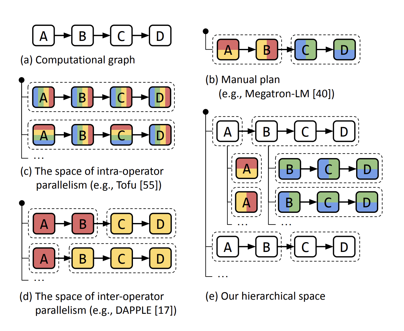
Parallel to these tradeoffs, the communication bandwidth on the device cluster also has an asymmetric nature. The intra-operator parallelism can use the high communication bandwidth, while the inter-operator parallelism is handled between distance devices with relatively lower bandwidth. The joint execution plan may not be globally optimal, it obtains high performance across different large models.
Alpa essentially is a compiler for parallel execution plans that partitions the cluster into device meshes based on the bandwidth hierarchy and performs inter-operator and intra-operator splitting.
Background
As mentioned previously, the authors consider a new view of ML parallelism that differs from the conventional views. Previously, the parallelism was one of the following types
-
Data parallelism - Data is distributed, but the model is replicated. The parameter updates are synchronized before the next iteration.
-
Operator parallelism - When the models are too large to fit in a device, the operators involved are split across the non-batch axes and the computations are performed in parallel across devices. This method usually requires large amount of communication across devices. When the tensors are partitioned evenly, i.e., SPMD, all devices follow the same communication patterns.
-
Pipeline parallelism - The model is split into stages which are placed on different workers. The training batch is split into microbatches for overlapped iterations of forward and backward passes across workers.
-
Hybrid parallelism - Researchers manually combined the above techniques to obtain much higher performance. One notable work is the Megatron-LM that optimizes the parallelization for transformer models (3D Parallelism).
-
Automatic combination of parallelism - Prior to this work, auto-parallelization was limited to combining data parallelism with at most one model parallelism approach missing improvement opportunities.
In contrast to this view, the authors consider inter-op and intra-op parallelisms as described before. With such a view, techniques such as Megatron-LM, ZeRO (that involves updates sharding) can be viewed as intra-op parallelism. On the other hand, techniques such as GPipe, 1F1B and PipeDream are all pipeline optimizations that come under inter-op parallelism. The authors of this paper adopt synchronous 1F1B for pipeline parallelism.
Method Overview
As mentioned previously, Alpa considers two-level planning
-
At the intra-op level, minimize the cost of executing a stage of the computational graph on a given device mesh (that have high bandwidth between each other)
-
At the inter-op level, minimize the inter-op parallelization latency with respect to slicing the model and mapping the stage-mesh pairs. The inter-op optimization depends on knowing the execution cost of each stage-mesh pair reported by the intra-op optimizer.
Alpa does this by generating an intermediate representation similar to Jax which is used by the optimization steps.
A device mesh is a 2-dimensional logical view of a set of physical devices (all having same compute capability) which communicate with different bandwidths in each dimension. We will delve deeper into the two stages below.
Intra-operator Parallelism
Alpa adopts the SPMD-style intra-op parallelism that partitions operators evenly across devices and executes the same instructions on all devices assuming that the devices in the mesh have equivalent compute capability. This decision greatly reduces the search space and unifies approaches such as data parallelism, ZeRO and Megatron LM. Alpa formalizes the problem as an integer linear programming problem.
The goal of intra-op pass is to pick one parallel algorithm for every operator to minimize the execution time of the entire graph. The authors use a sharding spec to define the layout of a tensor - each dimension of a tensor is S (sharded) or R (replicated). The partitioned tensor axes must be mapped to mesh axes.
Through this, we can succinctly represent different ways of partitioning a matmul.
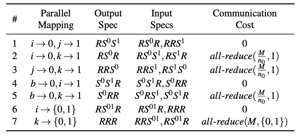
The model graph is represented in XLA’s HLO format, that summarizes common DL operators into less than 80 primitive operators whose parallel algorithms can be manually enumerated.
The ILP then considers the node and edge communication costs which can be solved by an off-the-shelf solver.
The equation is given by
\[\min_s \sum_{v \in V} s^T_v (c_v + d_v) + \sum_{(v, u) \in E} s^T_v R_{vu} s_u\]Although these different costs can be obtained by profiling, the authors suggest heuristic calculations to prevent executing multiple operators on the cluster wasting resources. There can be post-ILP optimizations similar to the ones in ZeRO to further improve the efficiency.
Inter-op Parallelism
Previous works consider a simplified problem where the device for each stage is pre-assigned and all stages have fixed data or operator parallelism plan. Alpa jointly optimizes everything considering a much general scenario.
The computational graph is split based on the topology order, and each stage has its own intra-op cost obtained from the intra-op pass. The cost is minimized considering the micro-batches inn the pipeline. The latency is given by
\[T^* = \min_{s_1, \dots, s_S} \left\{ \sum_{i = 1}^S t_i + (B - 1) \cdot \max_{1 \leq j \leq S} \{t_j\}\right\}\]The first term is the total latency of all stages, interpreted as the latency of the first micro-batch groin through the pipeline; the second term is the pipelined execution time for the rest of the micro-batches which is bounded by the slowest stage in the 1F1B pipeline.
Additionally, for an operator in the forward pass of the graph, the corresponding backward operator should be in the same submesh - the backward propagation usually uses the similar set of tensors during the forward pass, reducing the communication.
The authors formulate this as a DP formulation, cleverly considering primitive sub-mesh sizes to reduce the search-space significantly! These were the high level ideas, and there are considerations for cases where the operators do not fit into one device, etc. They introduce further techniques to prune the search space
-
Early pruning - Get rid of states that have higher cost than the current best
-
Operator clustering - Element-wise operators can be merged without much change in the cost. Greatly reduces the search space.
Parallelism Orchestration
Once the optimal assignment is found, XLA and GSPMD are used to generate parallel executables. Alpa implements additional parallelism orchestration pass to address cross-mesh communications. They introduce cross-mesh resharding for different sharding specs - P2P send/recv primitives.
Language Models are Few-Shot Learners
The paper from OpenAI that started it all. The after-effects of this work are still rapidly progressing. Let’s dive in.
The focus in NLP shifted from specialized models to task-agnostic systems for downstream applications. What started out as single layer representations, got converted to RNNs with multiple layers of representations and contextual states for stronger representations, and finally in the form of a transformer language model that seem to have amazing generalizing capabilities.
When this paper was proposed, people were still training these models on labeled datasets, and with the unavailability of large scale general datasets outside task-specific ones, developing a large generalizable model was a challenge. Furthermore, the narrowness of the datasets can also inhibit the capabilities of the model. The authors of this paper argue that humans do not require such large scale datasets to perform these general capabilities, and quickly learn from only a few demonstrations. To counter these limitations, the previous works experimented with meta-learning and scaling the size of the language models. The authors note the smooth trend in improvement with scale, and they double down on this hypothesis.
The largest model trained prior to this had 17B parameters. In this paper, the authors trained a 175B parameter model!
Approach, Model and Dataset
The pre-training of GPT follows a similar procedure to previous models at a larger scale. With this paper, they introduce new paradigms to evaluate/tune the model for in-context learning
-
Fine-tuning - Curating datasets for specific tasks for better performance. The authors mention that they don’t use this paradigm with GPT-3 to test it’s generalizing capabilities.
-
Few-Shot - Model is given a few input demonstrations as part of the prompt to adapt to a new task
-
One-shot - Same as above, but only one example if provided
-
Zero-shot - Testing the capabilities of the model for new tasks without providing any new demonstrations
The model architecture is same as GPT-2 that uses alternating dense and locally banded sparse attention patterns similar to Sparse Transformer.
Many datasets for language models rapidly expanded and culminated into the Common Crawl dataset consisting of nearly a trillion words. The authors improved the dataset by
-
Filtering based on similarly to a range of high-quality reference corpora
-
Fuzzy deduplication at the document level to prevent redundancy and preserve the integrity of the validation set
-
Addition of high-quality reference corpora into the training mix
One concern people have with large datasets is the memorization of downstream test tasks. To reduce this effect, the authors tried to remove all benchmark test instances from the training set. They mention that due to a bug they did not do this perfectly, and there was contamination in some cases.
Training and Evaluation Details
Previous works showed that larger datasets perform better with larger batch sizes and a smaller learning rate. The authors use a gradient noise scale during training to guide the choice of the batch size. They use model parallelism (both intra-op and inter-op) to reduce the peak memory usage. All models were trained on V100 GPUs from Microsoft.
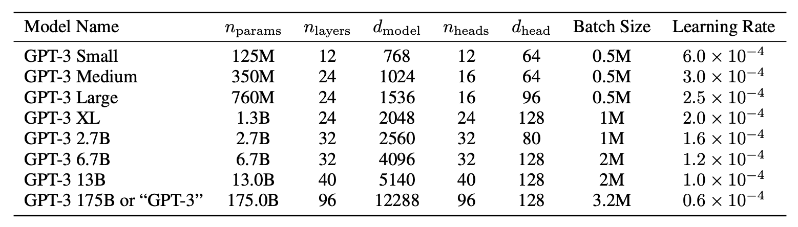
With this experiment, a strong paradigm in this field of research has been established - scaling both compute and model size has a power-law effect on the performance.
The authors test GPT-3 on multiple benchmarks carefully omitting cases that were a subset of the training dataset. They see that the few-shot setting achieves significantly higher performance that both one-shot and zero-shot. One-shot also shows improved performance with this model. in many cases, GPT-3 beat the SOTA model performance in multiple benchmarks. They test on generation, evaluation, reasoning and many other genres of tasks.
Limitations
The authors noticed that GPT-3 tends to repeat itself and in some cases the few-shot does not perform much better than one-shot inference. In a more architectural sense, they note that GPT-3 does not specifically cater to tasks with bidirectional language flow requirements. They also mention that large models such as these reach the limits of their pre-training objective that itself does not place importance on some task-specific needs. That is, more useful language systems may be better due to goal-directed actions rather than just making predictions. Furthermore, language models are not grounded in other forms of information such as video and audio.
Compared to humans, GPT-3 has much lower sample efficiency (it does meh with much much more samples seen during pre-training). Finally, both training and inference on such large models is very expensive and inconvenient. This has been changing in the recent times due to the advancements in RLHF and distillation techniques.
The authors also mention the broader impact of this paper, and warn the readers about the potential misuses of language models. The biases in the training datasets like certain stereotypes can propagate into the model and also about the energy due to the rise in this domain.
Training Compute-optimal Large Language Models
The paper tries to answer an important dilemma in training language models - is it better to train bigger models that are potentially undertrained or train smaller models on more data? The authors noted the trends in model and tried to derive an empirical law for the trends observed. They note that the budget for model training is known apriori, and the training can only be done once, estimating the best hyperparameters is critical.
So, the question we are concerned with is - Given a fixed FLOPs budget, how should one trade-off model size and the number of training tokens?
There have been some previous works around this. A 10x increase in the computational budget should increase 5.5x while the number of training tokens should only increase 1.8x. However, the authors note that the previous works did not consider the variations in tokens, learning rate schedule and other hyper-parameters to better model the behaviors.
Note. This work is mainly for dense transformer architectures. They mention that there are orthogonal works like RAG and MoE that improve the models, but the motivation for this paper is to understand the behavior of dense transformers.
Approach
In the first method, the authors tried to vary the number of training steps for a fixed family of models. They obtained the minimum loss achieved for a given number of training FLOPs. Using the interpolants, they obtain a mapping from any FLOP count C to most efficient model size N and training tokens D. They obtain the relationship \(N_{opt} \propto C^{0.5}\) and \(D_{opt} \propto C^{0.5}\) contradicting previous results.
In their second approach, they vary the model size for a fixed set of training FLOP counts and consider the final training loss for each point. It essentially answers the question for a given FLOP budget, what is the optimal parameter count. These are the IsoFLOPs experiments, and they obtain \(N_{opt} \propto C^{0.49}\) and \(D_{opt} \propto C^{0.51}\).
In the final approach, they modeled all the final losses considering the previous experiments, and considering a classical risk decomposition, they propose
\[\hat L(N, D) = E + \frac{A}{N^\alpha} + \frac{B}{D^\beta}\]-
The first term captures the loss for an ideal generative process on the data distribution and corresponds to the entropy of the natural text.
-
The second term captures the fact that a perfectly trained transformer with \(N\) parameters underperforms the ideal generative process.
-
The final term captures the fact that the transformer is not trained to convergence, as we only make a finite number of optimisation steps, on a sample of the dataset distribution.
To fit the empirical observations, they minimize a Huber loss on this formulation and also consider possible local minimas. Finally, they obtain the following results -
| Approach | Coeff. \(a\) where \(N_{\text{opt}} \propto C^a\) | Coeff. \(b\) where \(D_{\text{opt}} \propto C^b\) |
|---|---|---|
| 1. Minimum over training curves | 0.50 (0.488, 0.502) | 0.50 (0.501, 0.512) |
| 2. IsoFLOP profiles | 0.49 (0.462, 0.534) | 0.51 (0.483, 0.529) |
| 3. Parametric modelling of the loss | 0.46 (0.454, 0.455) | 0.54 (0.542, 0.543) |
| Kaplan et al. (2020) | 0.73 | 0.27 |
The key insights they obtain are -
-
The current language models are considerably over-sized given the compute budges.
-
The amount of training data that is projected to be needed is far beyond what is current used to train LLMs.
So the authors recommend that for a given training compute budget, smaller models should be trained on more tokens to achieve the most performant model.
Chinchilla
Considering the optimal hyperparameters they obtained, the authors trained a language model called Chinchilla as a competitor to Gopher. It is 4\(\times\) smaller than Gopher, and similarly the memory footprint and inference costs are reduced too. They follow a mixed-precision training procedure.
The results obtained are very impressive - Chinchilla significantly outperforms Gopher on many evaluation subsets.
Conclusion
The authors assert that scaling data instead of scaling models is the right way to obtain the best performance. We need to curate high-quality data - current models (e.g., GPT-3, MT-NLG) use only ~300B tokens, far below optimal recommendations (e.g., 1.5T tokens for 70B models).
They mention that such results and methodologies can also be extended to other kinds of models outside autoregressive language models.
Overall, this paper pushes towards an experimental based theoretical analysis of models and establishes a framework for compute-optimal training, demonstrating that equal scaling of parameters and tokens maximizes model performance. Chinchilla validates this hypothesis, achieving SOTA results with reduced computational overhead. Future work must prioritize dataset quality and ethical considerations alongside scaling.
Flash Attention
One of the seminal papers that has significantly reduced the energy usage of these large transformer models. At the core of transformers is the attention mechanism that becomes a bottle neck for long sequences. Both the time and space complexity scale quadratically with the sequence length making it infeasible to work with long context. Some previous works tried to reduce these requirements using sparse-approximations, low-rank approximations and other niche techniques which did not gain traction. The issue is that they reduce the FLOPs but because of the behavior of GPUs, this does not necessarily translate to optimized run-times.
Flash Attention on the other hand leverages the various hierarchies in the GPUs to utilize the resources most efficiently (to their fullest extent) and reduce both time and space requirements. Due to the reduction of these requirements, they claim fast model training, higher quality models and SOTA attention speed.
Background
The GPU memory hierarchy has memory of different sizes and speeds. For example, the A100 GPU has 40-80GB of high bandwidth memory (HBM) with bandwidth 1.5-2.0TB/s and 192KB of on-chip SRAM per each of 108 streaming multiprocessors with bandwidth estimated around 19TB/s.

The on-chip SRAM is an order of magnitude faster than HBM but many orders of magnitude smaller in size. As compute has gotten faster relative to memory speed, operations are increasingly bottlenecked by memory (HBM) accesses. With this motivations, the authors exploit fast SRAM for Flash Attention.
As mentioned previously in these articles, GPU operations can be classified as compute bound (time is arithmetic operations dominant) or memory bound (time is memory access dominant). Memory bound operations have been optimized with the use of kernel fusion - multiple operations can be done with single load from HBM. It turns out that attention is a memory-bound operation since it mostly consists of element-wise operations.

In standard attention, the matrices \(S = QK^T\) and \(P = \text{softmax}(S)\) are explicitly calculated using up \(\mathcal O(N^2)\) memory. In terms of GPU usage, it looks like this -
-
Load \(Q, K\) by blocks from HBM, compute \(S = QK^T\), write \(S\) to HBM.
-
Read \(S\) from HBM, compute \(P = \text{softmax}(S)\), write \(P\) to HBM.
-
Load \(P\) and \(V\) by blocks from HBM, compute \(O = PV\), write \(O\) to HBM.
We shall now see how Flash Attention improves on this with kernel fusion
Method
The main idea is that, like matrix multiplication, \(Q, K, V\) can be split into blocks to load from slow HBM to fast SRAM.
Forward Pass
Tiling. The main hurdle in the previous works was getting softmax to work with tiling mechanisms. how can softmax be fused across blocks? Since we apply softmax across columns of \(K\), for each column, we can maintain \(f(x) = e^{x - m(x)}, l(x) = \sum_i f(x)_i\) to calculate the softmax as \(f(x)/l(x)\) - they essentially keep track of the sum and maximum of elements (for numerically stable softmax). These two statistical quantities are calculated across blocks recursively all the way up to calculate the final softmax - forward pass of the flash attention algorithm.

Let us dive into a bit more detail. The output matrix \(O\) is stored in the HBM, and updates are made to store the correct output at the end of all block computations. For simplicity, let us consider blocks of sizes \((n \times d)\) where \(n\) is some factor of \(N\).
-
In typical softmax \(O_ij = \underbrace{\sum_k Q_{ik} K_{kj}}_{S^i} \cdot V_j\) (using superscript for row and subscript for column). In Flash attention, we pick up block \(Q_{b_i}\) and \(K_{b_j}\), perform the multiplication to obtain a sub-matrix \(S_{b_ib_j}\) of size \(n \times n\) and store
-
\(m^k_{b_ib_j}\) - The maximum value of each row vector.
-
\(l^k_{b_ib_j}\) - Sum of \(e^{S_{b_ib_j} - m^k}\) across all the columns in each row
-
-
We compute the result \(f(S_{b_ib_j})V_{b_i}\) with appropriate softmax values using the \(m, l\) values and update the corresponding \(n \times d\) block in \(O\). Remember that this is the partial result and needs to updated with further calculations.
-
When another partial sum for the block in \(O\), the entry can be easily updated with the new \(m, l\) values (the math is super easy) to calculate the softmax of the complete partial sum so far.
Although the asymptotic time complexity is still the same, the constant associated would decrease significantly due to lower HBM accesses. The space usage increases by \(2*N\) while dropping the intermediate results that occupy \(\mathcal O(N^2)\)! This is huge! The time computation becomes \(\mathcal O(N^2d^2 M^{-1})\) where \(M\) is the size of SRAM, as compared to \(\mathcal \Omega (Nd + N^2)\).
Input:
-
Matrices \(Q, K, V \in \mathbb{R}^{N \times d}\) in HBM.
-
On-chip SRAM of size \(M\).
-
Softmax scaling constant \(\tau \in \mathbb{R}\).
-
Masking function \(mask\).
-
Dropout probability \(p_{drop}\).
Steps:
-
Initialize the pseudo-random number generator state \(R\) and save to HBM.
-
Set block sizes:
- \(B_c = \left\lfloor \frac{M}{4d} \right\rfloor\),
- \(B_r = \min\left(\left\lfloor \frac{M}{4d} \right\rfloor, d'\right)\).
- Initialize in HBM:
- \(O = (0)^{N \times d} \in \mathbb{R}^{N \times d}\),
- \(\ell = (0)^N \in \mathbb{R}^{N}\),
- \(m = (-\infty)^N \in \mathbb{R}^{N}\).
- Divide \(Q\) into
\(T_r = \left\lceil \frac{N}{B_r} \right\rceil\) blocks
\(Q_1, Q_2, \dots, Q_{T_r}\) of size \(B_r \times d\) each, and divide both \(K\) and \(V\) into
\(T_c = \left\lceil \frac{N}{B_c} \right\rceil\) blocks
\(K_1, K_2, \dots, K_{T_c}\) and
\(V_1, V_2, \dots, V_{T_c}\) of size \(B_c \times d\) each.
- Divide:
- \(O\) into \(T_r\) blocks \(O_1, O_2, \dots, O_{T_r}\) of size \(B_r \times d\) each,
- \(\ell\) into \(T_r\) blocks \(\ell_1, \ell_2, \dots, \ell_{T_r}\) of size \(B_r\) each,
- \(m\) into \(T_r\) blocks \(m_1, m_2, \dots, m_{T_r}\) of size \(B_r\) each.
- For \(j = 1 \text{ to } T_c\) do:
1. Load \(K_j, V_j\) from HBM to on-chip SRAM.
2. For \(i = 1 \text{ to } T_r\) do:
1. Load \(Q_i, O_i, \ell_i, m_i\) from HBM to on-chip SRAM.
2. On-chip, compute
\(S_{ij} = \tau\, Q_i\, K_j^T \in \mathbb{R}^{B_r \times B_c}\).
3. On-chip, compute
\(S^{masked}_{ij} = mask(S_{ij})\).
4. On-chip, compute:
- \(\tilde{m}_{ij} = \text{rowmax}(S^{masked}_{ij}) \in \mathbb{R}^{B_r}\),
- \(\tilde{P}_{ij} = \exp\Bigl(S^{masked}_{ij} - \tilde{m}_{ij}\Bigr) \in \mathbb{R}^{B_r \times B_c}\) (pointwise),
- \(\tilde{\ell}_{ij} = \text{rowsum}(\tilde{P}_{ij}) \in \mathbb{R}^{B_r}\).
5. On-chip, compute:
- \(m^{new}_i = \max(m_i, \tilde{m}_{ij}) \in \mathbb{R}^{B_r}\),
- \(\ell^{new}_i = e^{\,m_i - m^{new}_i}\,\ell_i + e^{\,\tilde{m}_{ij} - m^{new}_i}\,\tilde{\ell}_{ij} \in \mathbb{R}^{B_r}\).
6. On-chip, compute
\(\tilde{P}^{dropped}_{ij} = dropout\Bigl(\tilde{P}_{ij},\, p_{drop}\Bigr)\).
7. Write to HBM:
\(O_i \gets \text{diag}(\ell^{new}_i)^{-1}\Bigl(\text{diag}(\ell_i)\,e^{\,m_i - m^{new}_i}\,O_i + e^{\,\tilde{m}_{ij} - m^{new}_i}\,\tilde{P}^{dropped}_{ij}\,V_j\Bigr)\).
8. Write to HBM:
\(\ell_i \gets \ell^{new}_i,\quad m_i \gets m^{new}_i\).
3. End For (over \(i\)).
-
End For (over \(j\)).
-
Return \(O, \ell, m, R\).
Block-Sparse FlashAttention
In vanilla attention mechanisms, a mask is typically applied to the output after all the intermediate computations are completed. If the matrices are manipulated during the calculations, we may underutilize the GPU and lead to a less efficient computation.
Flash Attention solves this problem to some extent - it defines block sparsity masks for each block and extends the previous algorithm by simply considering blocks that have non-zero mask! This speeds-up computations a lot!
Backward Pass
Recomputation. Instead of explicitly storing the intermediate matrices, the authors suggest gradient checkpointing for backward pass of attention. Peculiarly, gradient checkpointing speed-up the backward computation due to lower HBM accesses even though the intermediate matrices have to be recomputed.
Essentially, again, instead of storing \(P, S\) both of which are \(\mathcal O(N^2)\), we simply load \(K, Q, V\) that have the size \(N \times d\) and recompute the required results for backward pass. The key ideas for gradient computations are very similar to the forward pass (more complicated because of too many computations).
Summary
In accordance with their claims, the authors show the following results -
-
Fast models - BERT trains 15% faster and \(3\times\) end-to-end speedup compared to typical architectures for GPT-2. Only \(1.7\times\) speedup compared to Megatron-LM.
Can FlashAttention be combined with Megatron-LM? I think so, need to read this up.
-
Better Models with Longer Sequences - The context length of \(GPT-2\) can now be increased \(4\times\) and the training is still faster than Megatron-LM!
-
Benchmarking Attention -

So that concludes our analysis on FlashAttention. The authors also mention some limitations -
-
Developing new CUDA kernels for each hardware! Projects like Triton and other DSLs like TVM are helping with these issues though.
-
The authors did not discuss how to extend these techniques to distributed systems. Later works, FlashierAttention and FlashAttention3 extended this work to further improve the efficiency.
This is another good blog explaining Flash Attention well. Look into this if what I wrote does not make sense!
Paged Attention
Running LLM services is very expensive. It is imperative we ensure the LLM serving systems are efficient and have a high throughput. KVCache made a profound impact on the efficiency of LLMs by storing the previously generated keys and values during the decoding process.
An LLM generates tokens in an autoregressive manner, and this sequential generation process makes the workload memory-bound. We need to efficiently manage memory to load more number of batches and increase the throughput.
In a serving system, typically 30% of the memory is used to store the states for the requests. The KVCache for these different requests are often stored precariously resulting in almost 60-80% of the storage going towards fragmentation and reservation spaces (since these tensors are stored in contiguous memory). As a result, the GPU is underutilized because the batch sizes are limited.

This work draws inspiration from OS memory management to improve the efficiency of KV Cache memory storage, resulting in storage of higher batches and consequently higher throughput.
Contiguous memory storage has become a standard in deep learning systems. However, the dynamic nature of the tokens generated over time make the existing systems inefficient due to pre-allocation and not being able to share the memory. For example, decoding algorithms such as parallel sampling and beam search, the generated sequences partially share the KV cache and the current systems do not support memory sharing due to contiguous storage.
PagedAttention addresses these limitations by storing KV cache in a flexible manner similar to OS virtual memory - with logical memory and pages.
Background
-
Batching multiple requests. Since the input tokens and the generated tokens vary and are not known apriori, batching them together is a difficult task. However, the MLPs in the transformer layers are token-agnostic allowing different requests to be batched for this stage of the decoding process. In such manner, continuous batching is employed where the self-attention of the requests are processed independently on different GPUs and the requests are then merged for the forward pass through MLP.
-
The lifetime of a request can be classified into prompt phase (where the prompt is processed as a whole) and the decoding phase (token generation in autoregressive manner). The prompt phase of the requests can be efficiently parallelized across GPUs.
-
The size of the KV Cache grows very quickly. With more powerful GPUs, the FLOPs typically increase dramatically while the memory improves incrementally. Therefore, memory would be a significant bottleneck going forward.
Memory Management in KV Cache

As we mentioned before, KV Cache is stored as a contiguous tensor, and a chunk of memory is pre-allocated statically irrespective of actual input or eventual output length of the request. As a result, there are three primary sources of memory wastage
-
Internal fragmentation - Over-provisioning for potential maximum sequence lengths
-
Reserved slots for future tokens. Although this maybe used in the future, it could be used now for holding other requests.
-
External fragmentation from the memory allocator.
Method
PagedAttention allows storing continuous keys and values in non-contiguous memory space. It partitions KV cache of each sequence into KV blocks and each block contains the key and value vectors for a fixed number of tokens based on the Block Size B. During the attention computation, the PagedAttention kernel fetches different KV blocks separately.
The memory manager is analogous to virtual memory in operating systems - the KV cache is represented as a series of logical KV blocks, filled from left to right. The unfilled positions on each row are reserved for future generations. On GPU workers, a block engine allocates a contiguous chunk of GPU DRAM and divides it into physical KV blocks and maintains block tables (mapping between logical and physical KV blocks). Note that the block size is an important hyperparameter that is a trade-off between spaces reserved for the future and the block table overhead.

The whole reason we maintain contiguous blocks is to ensure faster retrieval, right?
New physical blocks are assigned only when all the previous blocks for a request are full.
Due to the flexible nature of this memory management, other decoding techniques like parallel decoding, beam search and shared prefix become much more efficient.
-
In parallel decoding a single physical block and be mapped to multiple logical blocks (tracked through a reference count). Here only the initial prompt blocks are shared
-
In beam search, blocks other than the prefill phase are shared and a block tree has to be generated similar to OS process tree. Previous systems maintained copies of KV cache for beam candidates and this technique prevents that.
-
In case of system prompts (usually very long), LLM service providers usually have a single copy for the tokens, and the same system can be adapted to PagedAttention as well
When the number of requests surpass the system’s capacity, the authors adopt a FCFS policy. There are two main questions that need to be answered -
-
What blocks need to be evicted? They use an all-eviction policy where all the blocks relating to a request are evicted.
-
How to recover evicted blocks? The evicted blocks are copied to the CPI memory, and swapped based on the requirement
They also adopt a recomputation technique if the latency is much lower.
Distributed Execution. When multiple GPUs are present, the memory manager needs to be capable of handling distributed memory. They implement the memory management in a Megatron-LM style tensor model parallelism. Each model shard still processes the same set of input tokens, thus requiring the KV cache for the same positions - so a single KV cache manager within the centralized scheduler suffices.
Execution and Results
PagedAttention introduces memory access patterns that are not efficiently supported by the existing systems. They implemented their own GPU kernels
1) Fused re-shape and block write
2) Fusing block read and attention
3) Fused block copy
PagedAttention obtains significantly better throughput - It is able to handle 2-3x higher number of requests

The authors also performed a detailed ablation study for
-
Custom kernel operations - 20-26% lower latency
-
Block size - If the block size is too small, vLLM may not fully utilize the GPU’s parallelism for reading and processing KV cache. If the block size is too large, internal fragmentation increases and the probability of sharing decreases

-
Comparison of recomputation and swapping - depends on the PCIe bandwidth
Conclusion
It must be noted that these techniques work well for LLMs because they are memory bound. In other words, other DNN workloads may not see similar improvements because they tend to be compute-bound.
Furthermore, due to the significance of the transformer architecture, numerous specialized serving systems for it have been developed. There are other works like Orca that developed orthogonal techniques to improve GPU utilization.
Enjoy Reading This Article?
Here are some more articles you might like to read next: