Stable Diffusion Models
A brief introduction to image synthesis applications, stable diffusion models and its applications.
Image Synthesis
- Artificially generating images with some desired content
- Typically provided with some prompts for generation
- Multi-modal generation
- Generative models as solutions -
- Guided Synthesis
- Image editing
Previous Work
Generative Adversarial Networks
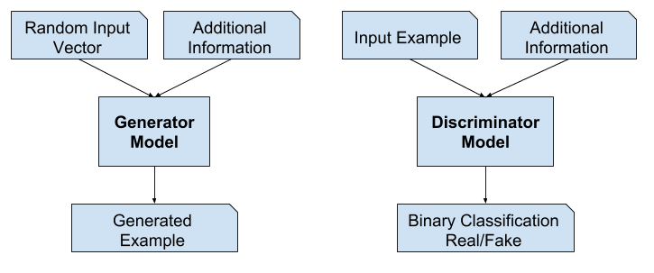
A Generative Adversarial Network consists of a generator and a discriminator pair to synthesize images representative of the dataset. These two ‘agents’ compete against each other, and try to optimize opposite cost functions. The generator is responsible for creating synthetic data that should resemble the real data from a specific dataset, such as images, audio, or text. The discriminator, on the other hand, evaluates the data it receives and tries to distinguish between real data from the dataset and fake data generated by the generator.
A variant of GANs, called conditional GANs operate in a latent space. That is, we have multi-dimensional space where each point corresponds to a set of parameters that can be mapped to data in the target distribution. The generator is then ‘conditioned’ on a random vector sampled from this latent space as input. These vectors act as a source of randomness that the generator uses to produce diverse data samples. By exploring different points in the latent space, the generator can generate a wide variety of data, allowing it to produce novel and creative outputs.
GANs
The loss function for a Generative Adversarial Network (GAN) consists of two components: the generator loss and the discriminator loss. Here’s the LaTeX code for the GAN loss function:
\[\mathcal{L}_{\text{GAN}}(G, D) = \mathbb{E}_{x \sim p_{\text{data}}(x)}[\log D(x)] + \mathbb{E}_{z \sim p_z(z)}[\log(1 - D(G(z)))]\]In this equation:
- \(\mathcal{L}_{\text{GAN}}(G, D)\) represents the GAN loss.
- \(G\) is the generator network.
- \(D\) is the discriminator network.
- \(x\) represents real data samples drawn from the true data distribution \(p_{\text{data}}(x)\) .
- \(z\) represents noise samples drawn from a prior distribution \(p_z(z)\) .
- \(G(z)\) is the generator’s output when given noise \(z\) .
- \(D(x)\) represents the discriminator’s output when given a real data sample \(x\) .
- \(1 - D(G(z))\) represents the discriminator’s output when given a generated sample \(G(z)\) .
The goal of training a GAN is to find the generator and discriminator that minimize this loss function. The generator aims to generate data that fools the discriminator (maximizing the second term), while the discriminator aims to distinguish between real and generated data (maximizing the first term). This adversarial training process leads to the generation of realistic data by the generator.
Issues
- Mode collapse - The process of training prompts generator to find one plausible example
- Monotonous output/Lack of diversity - unable to capture the complete dataset
- Difficult to optimize, unstable training, vanishing gradient
Diversity and Fidelity tradeoff
Cost functions may not converge using gradient descent in a minimax game
AutoRegressive (AR) Transformers
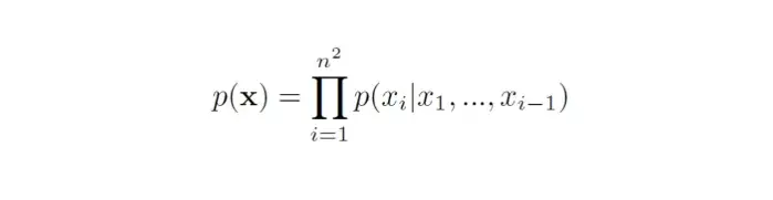
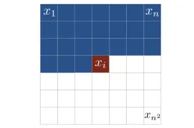
AR models treat an image as a sequence of pixels and represent its probability as the product of the conditional probabilities of all pixels
Models inherently forced to capture entire distribution unlike GANs
Allows us to use Likelihood Maximization
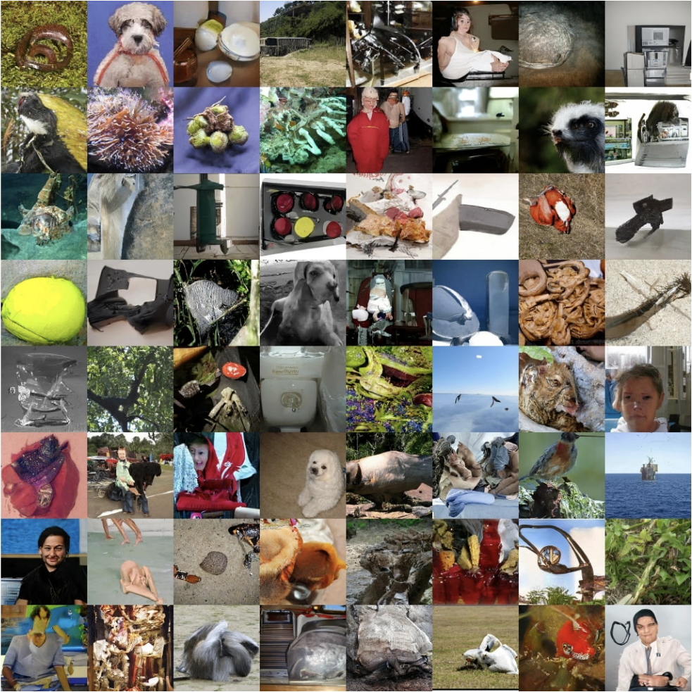
Not very high-resolution images due to memory constraints
Stable training process as compared to GANs
DALL-E uses transformers
pixelCNN
- Issues -
- Accumulated errors - Since pixels generated in sequence
- Computationally Expensive
- Pixel based
- Likelihood maximization unnecessary
- Captures barely perceptible\, high frequency details
Diffusion Models
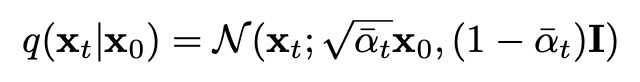
Destroy training data by adding noise to generate Gaussian noise.
Then learn to recover the data by reversing this process
A Diffusion Model is trained by finding the reverse Markov transitions that maximize the likelihood of the training data.
x0 is the image and xT is the noise!

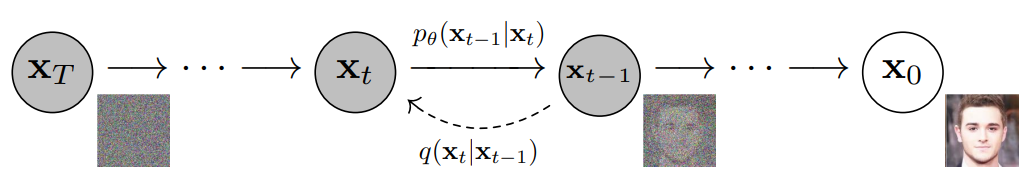
T is in the order of 1000s
β’s are progressively increased typically to make xT pure Gaussian
Smaller variances are preferred for better posterior estimation
With a large number of steps - process is reversible - mathematically shown
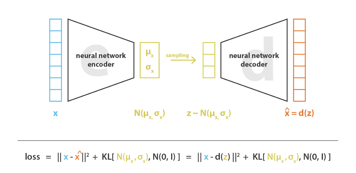
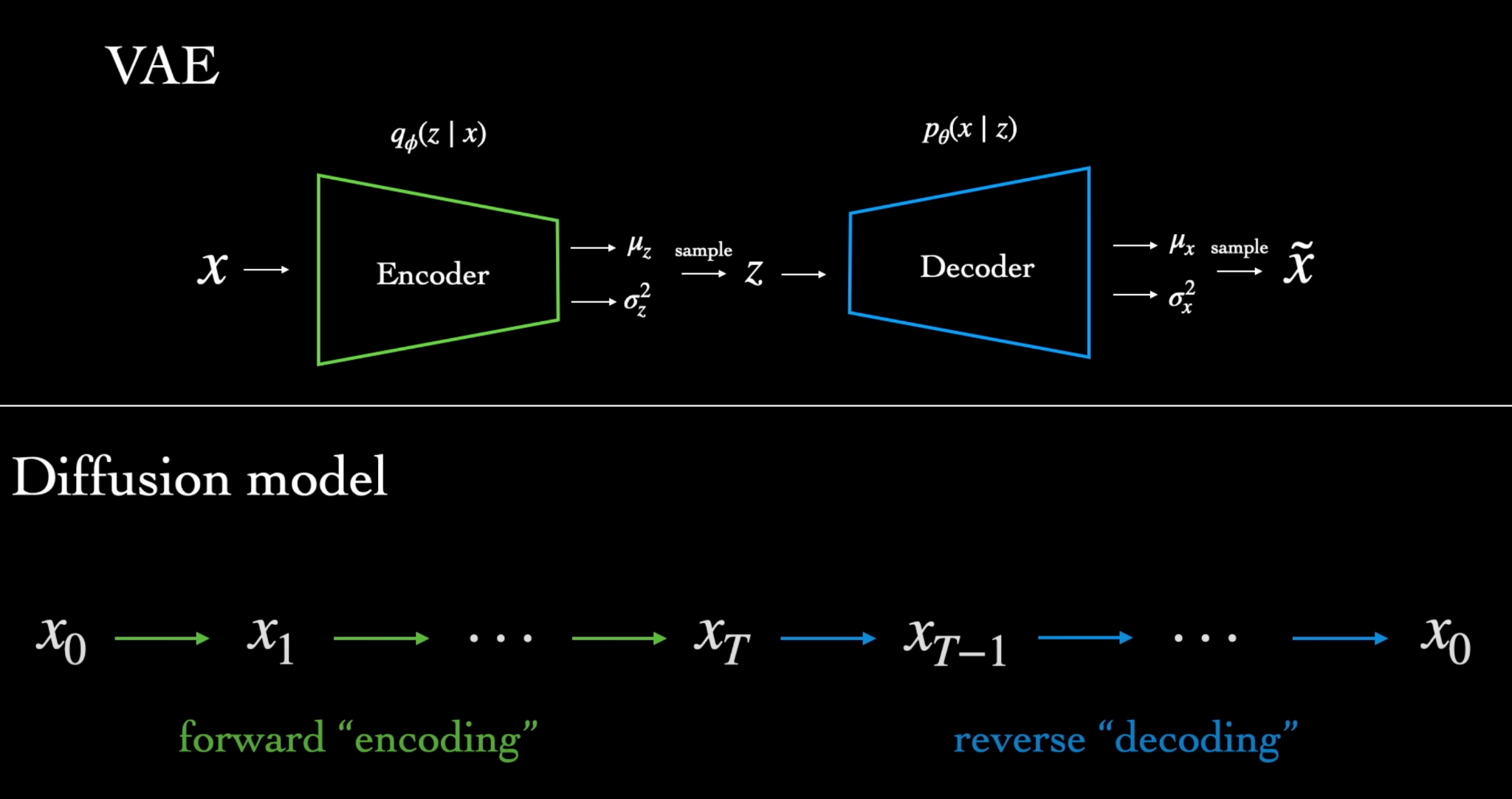
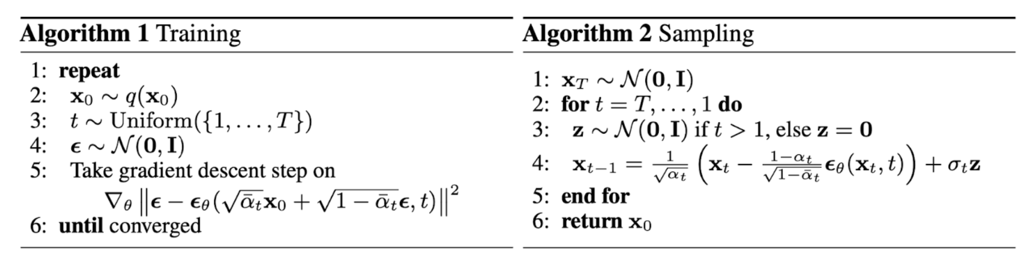
Training motivated from VAEs

T is in the order of 1000s Explain with diagram 2nd point Single network needed for diffusion models since forward process is fixed in DMs
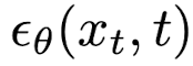
__Reverse Diffusion __ - The parameters have to be learned via a neural network
Encoder-Decoder type architecture

https://arxiv.org/pdf/2006.11239.pdf
T is in the order of 1000s Explain with diagram https://arxiv.org/pdf/2006.11239.pdf
Forward process allows sampling at an arbitrary _t _
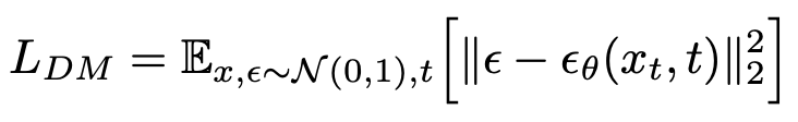
This allows efficient training using stochastic gradient descent for optimizing random terms
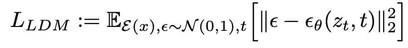
The simplified cost function in diffusion models is - \(DDPM\)
The model learns the data distribution p \(x\) by denoising a normal variable
These can be interpreted as a sequence of denoising autoencoders
https://arxiv.org/pdf/2006.11239.pdf
Difference from GANs
Not adversarial
Not in latent space
How is t added? Check out this paper
Inductive bias of images via U-Net architecture
Latent space captures low-level features and up-scales them
Skip connections preserve the high-level features
-
Advantages -
-
Stable from mode collapse - since based on likelihood
-
Smooth distribution due to diffusion
-
-
Disadvantages -
-
Computationally very expensive - repeated evaluations. 5 days on A100 GPU
-
Image generation time is high
-
Variational encoder - makes distribution U Nets are encoder decoder with skip connections
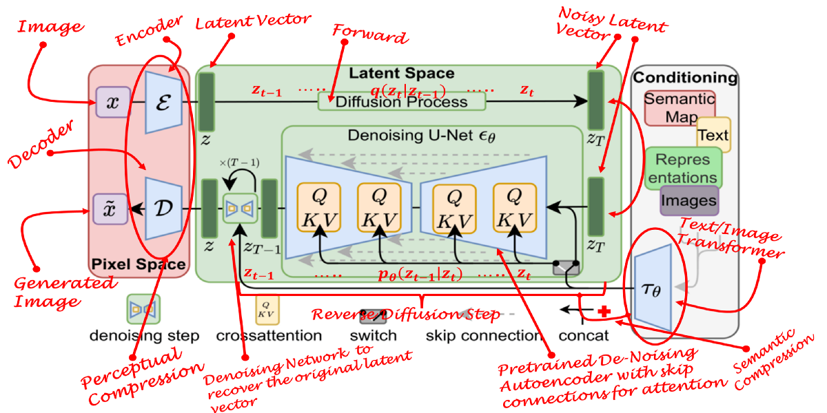
Latent Diffusion Models
- Denoising every pixel is unnecessary and computationally expensive.
- Work in the __latent space __ to deal with lower dimensions
- Image generation done in two-steps
- The perceptual compression stage removes high-frequency details
- Generative model learns the semantic variation in __semantic compression __ stage
- __Motivation - __ Perceptually equivalent but computationally suitable space
- Advantages
- Autoencoding done only once and various diffusion models can be explored
- Other conditional generation tasks
Features
High-resolution synthesis of images
Application to multiple tasks such as unconditional image synthesis\, inpainting\, stochastic super-resolution
General-purpose conditioning mechanism based on cross-attention\, enabling multi-modal training
Variable compression rate for the latent space
Latent space once generated\, can be used for multiple DM models
Latent Spaces - Autoencoding
Explicit separation of compressing and generation stages
Exploit the inductive bias of DMs in the latent space via U-Nets due to perceptual equivalence
Process
Given an image _x _ in RGB\, the encoder E encodes the image into z = E \(x\)
Encoder downsamples the image by a factor of f
Decoder D\, reconstructs image from latent space as x’ = D \(z\) = D \(E\)x\(\)
Stable Diffusion Models
Refined version of LDMs
Employ a frozen CLIP text encoder\, allowing it to generate images based on text prompts
Contrastive Language-Image Pre-Training
Generates text and image embeddings
Images and relevant text will have similar representations
A neural network trained on a variety of \(image\, text\) pairs
It can be instructed in natural language to predict the most relevant text snippet\, given an image\, without directly optimizing for the task
Zero-shot - model attempts to predict a class it saw zero times in the training data
An image encoder and a text-encoder
Attention
For conditioning the generation process
The prior is often either a text\, an image\, or a semantic map
A Transformer network encodes the condition text/image into a latent embedding which is in turn mapped to the intermediate layers of the U-Net via a cross-attention layer
Attention mechanism will learn the best way to combine the input and conditioning inputs in this latent space
These merged inputs are now the initial noise for the diffusion process.
Experiments
Perceptual Compression Tradeoffs
The downsampling factor in the universal autoencoder has to be chosen
Low downsampling factors \(1\, 2\) result in slow training progress - the diffusion model has to do the compression job
High factors cause stagnating fidelity after comparably few training steps - sample quality is limited due to information loss
Factors 4\, 8 and 16 strike a good balance
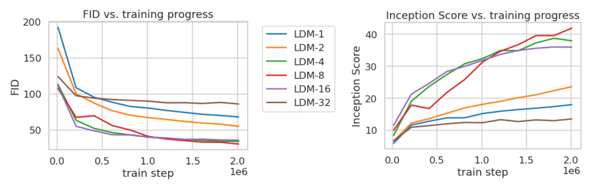
Image Generation
This model has half the parameters and requires 4 times lesser computation resources!
Precision and recall to assess the mode-coverage
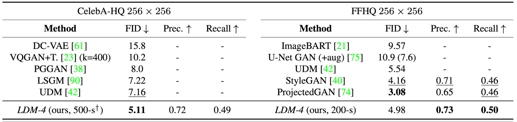
Precision and recall estimated by nearest neighbours
Conditional Tasks
Transformer Encoders for LDMs
For text-to-image generation\, BERT-tokenizer is used to infer a latent code that is mapped into the U-Net via cross-attention
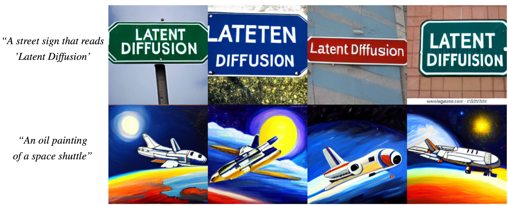
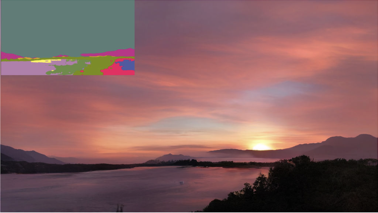
Image-to-Image translations
Semantic representations in the latent spaces are simply concatenated
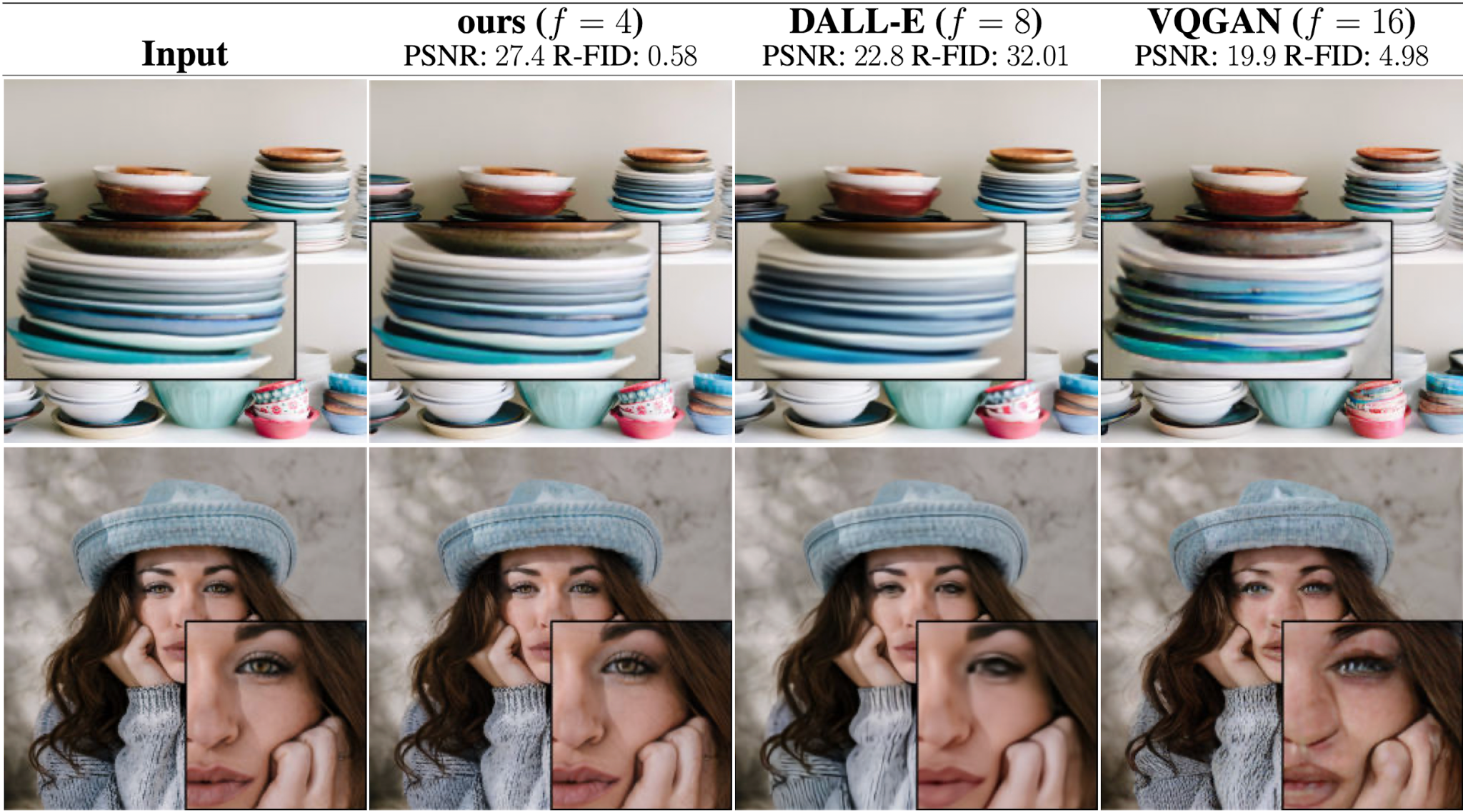
Super-Resolution
The low-resolution image is simply concatenated as the conditioned input after bi-cubic interpolation
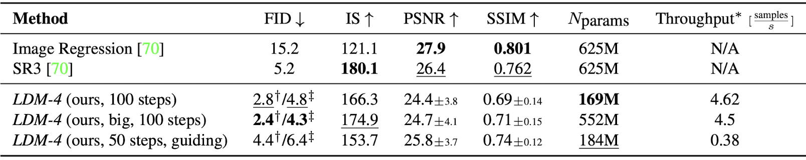
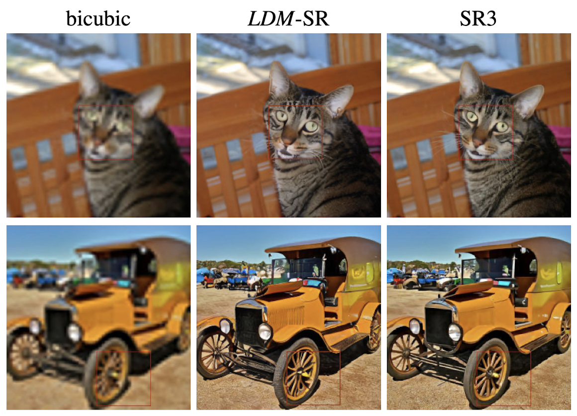
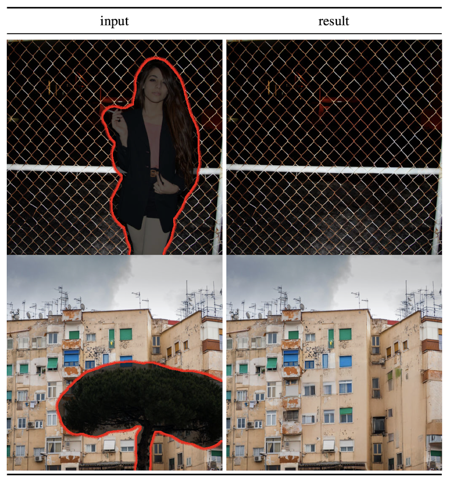
Image Inpainting
Summary
- Generative Models
- Autoregressive Transformers
- GANs
- Diffusion Models
- DMs
- Principles
- Issues
- Latent Diffusion Models
- Latent Spaces and Perceptible Compression
- Cross-attention for multi-modal generation
- Open Source